Given two inputs, the intial state and the goal state, the AI will navigate to find the optimal solution of a series of actions
Agent is an entity that perceives its environment and acts upon that environment. For instance, this entity could be an AI program, the environment could be the state of a chess game, and the AI will determine the action under that state, in another word, how to take the next move
A configuration of an agent in its environment, also can be understood as the state of the game in a chess game
The state from which the search algorithm starts, the environment when the agent first kick in
All possible choices that can be made by an agent in a state
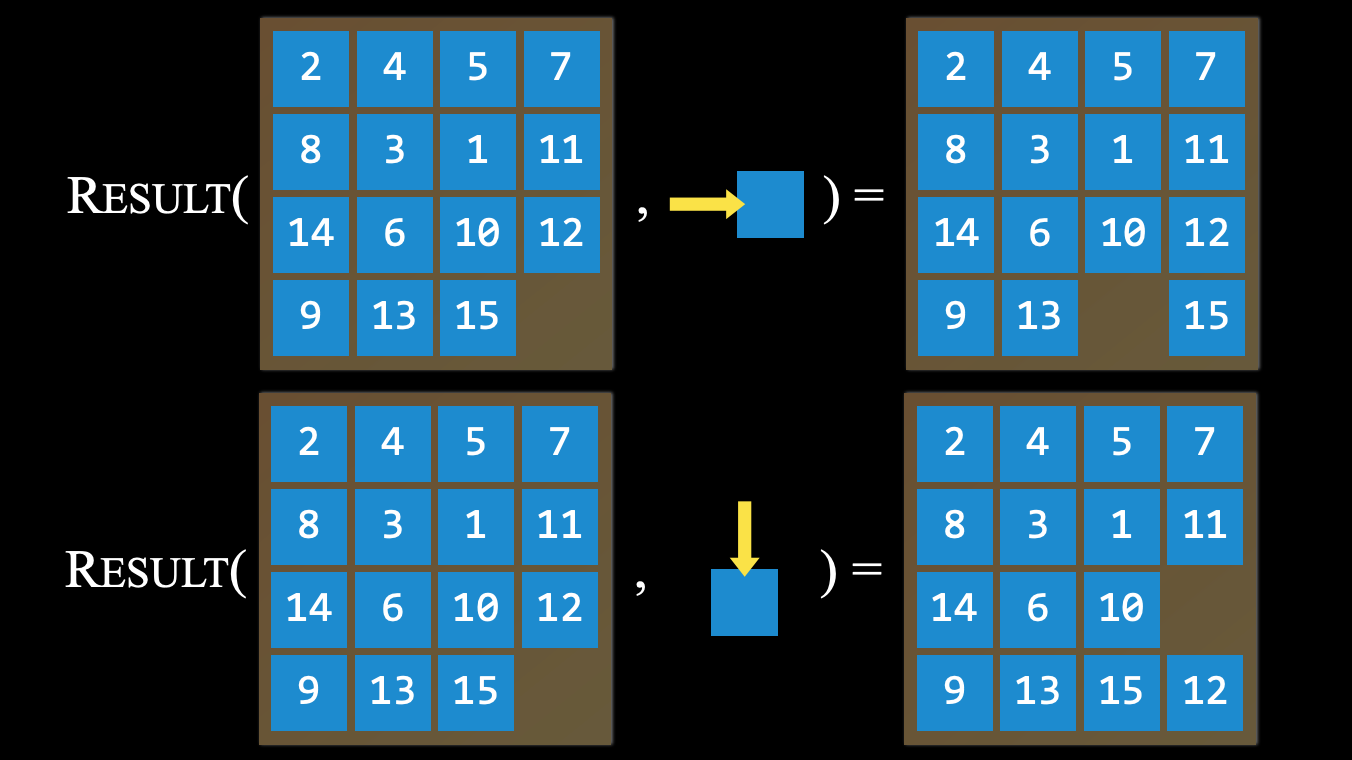
A description of what state results from performing any applicable action in any state
i.e. result(s, a) return the state in s by performing the action a
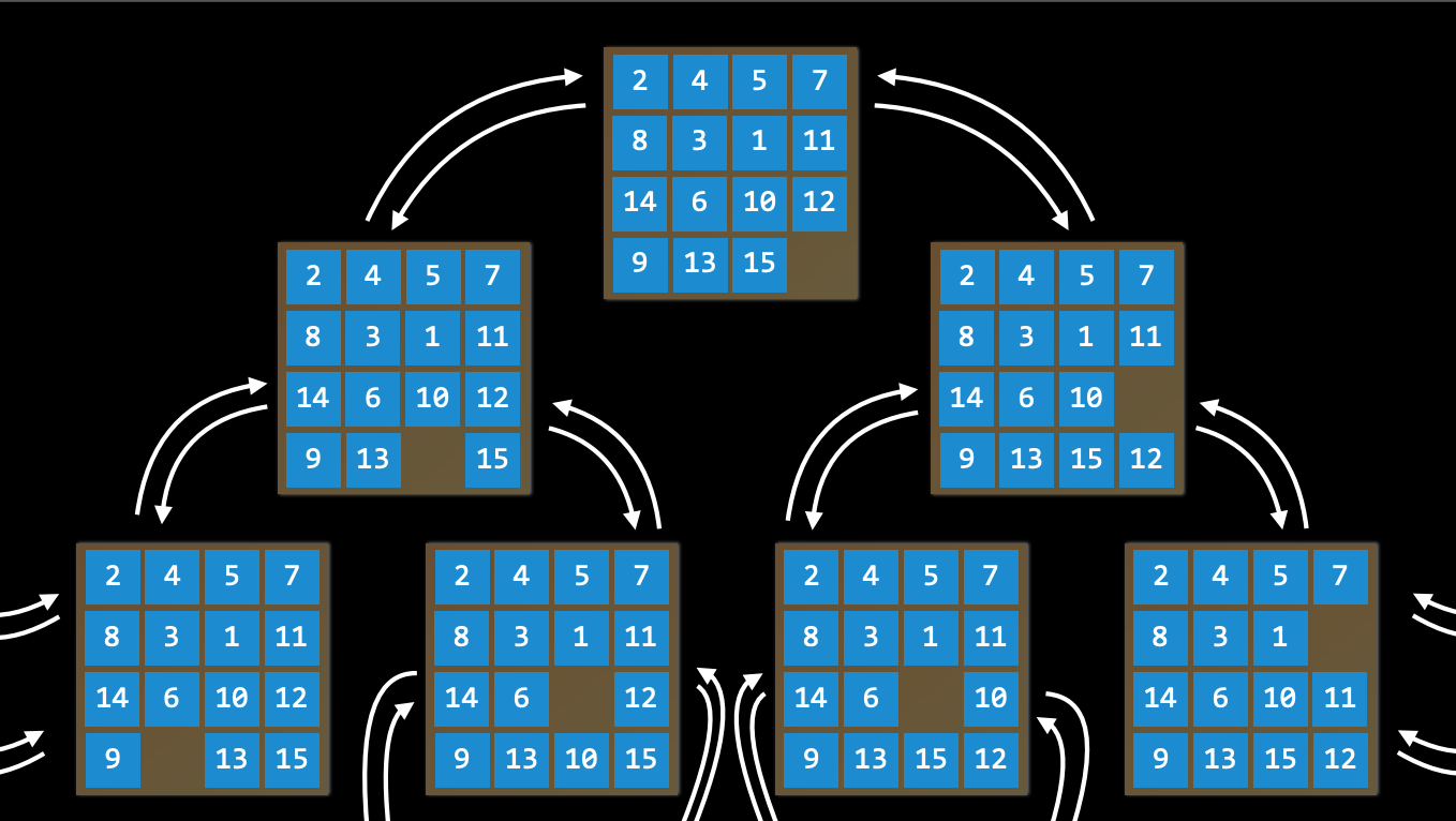
The set of all states reachable from the initial state by any sequence of actions
The condition that determines whether a given state is a goal state, if certain state passes the goal test, which means the algorithm should be terminated since we have found the solution
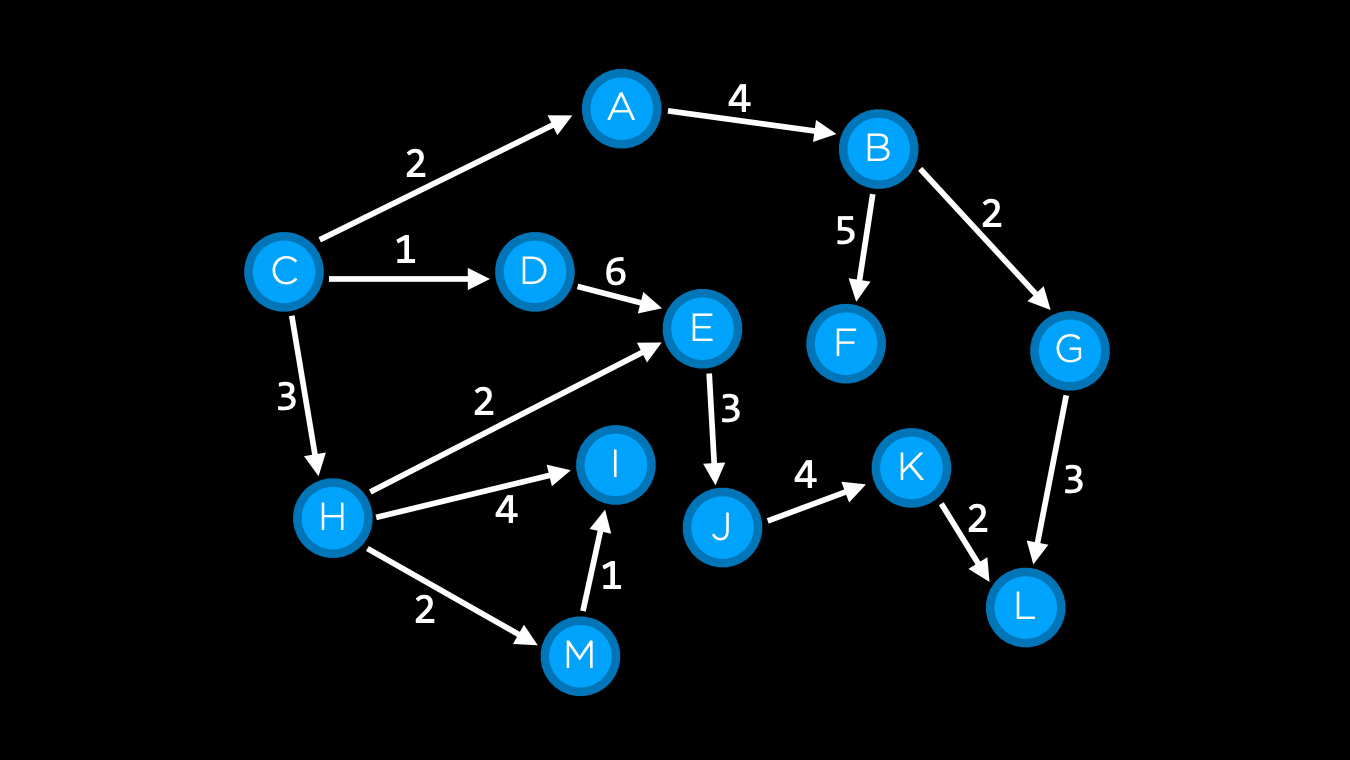
A numerical cost associated with a given path
The cost of each edge (between two vertices) could be 1 or more than 1
i.e. when navigating a path on the map, we do not only consider the distance but also trying to minimize the path cost, which in real life is the traffic condition on certain roads. If there's a bad traffic on a certain road, then the cost of that road is high
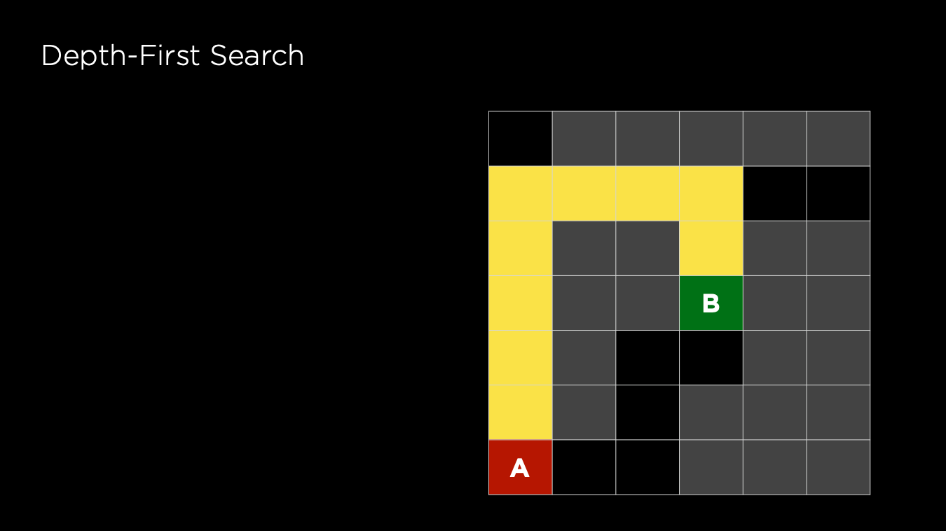
Exhausts each one direction before trying another direction. If there are several possible ways, the agent will choose randomly. So, DFS might not be efficient to find the path due to this randomness, and it does not guarantee to find the shortest path
For example:
OR
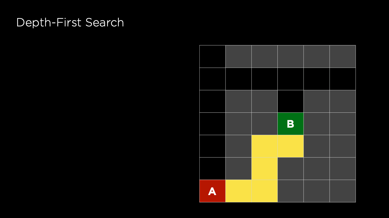
DFS typically uses a stack data structure to store all of the possible actions. Below is the pseudo code for the DFS implementation
DFS(G,v)   ( v is the vertex where the search starts )
    Stack S := {};   ( start with an empty stack )
    for each vertex u, set visited[u] := false;
    push S, v;
    while (S is not empty) do
        u = pop S;

        if u is destination then
            return path from v to u

        if (not visited[u]) then
            visited[u] = true;
            for each unvisited neighbour w of u
                push S, w;
Follow multiple directions at the same time, taking one step in each possible direction before taking the second step in each direction
Guarantee the shortest path, but takes relatively a long time as it seeks each directions setp by step. Also, BFS only considers unweighted path and ignore the path cost, so it's more efficient to use A* when doing map navigation rather than BFS
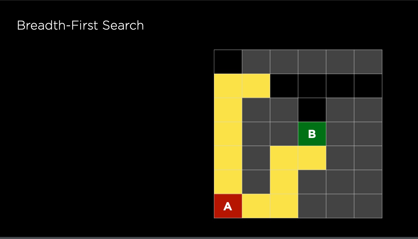
BFS typically uses a queue data structure to store all of the possible actions. Below is the pseudo code for the BFS implementation, the only difference between DFS and BFS is one uses stack and one uses queue
BFS (G, s)  (G is the graph and s is the source node)
    let Q be queue
    Q.enqueue( s )
    mark s as visited

    while ( Q is not empty)
        v  =  Q.dequeue( )

        if v is destination then
            return path from s to v

        for all neighbours w of v in Graph G
            if w is not visited
                Q.enqueue( w )
Check out examples directory for Python implementation of DFS and BFS that solves mazes
At any time, choose the state that is closest to the goal as the next state (only consider the estimated cost to the goal), as estimated by a heuristic function h(n). However, it only consider the distance between the current node to the destination but not the cost to reach this node from the source. The greedy algorithm does not guarantee the shortest path
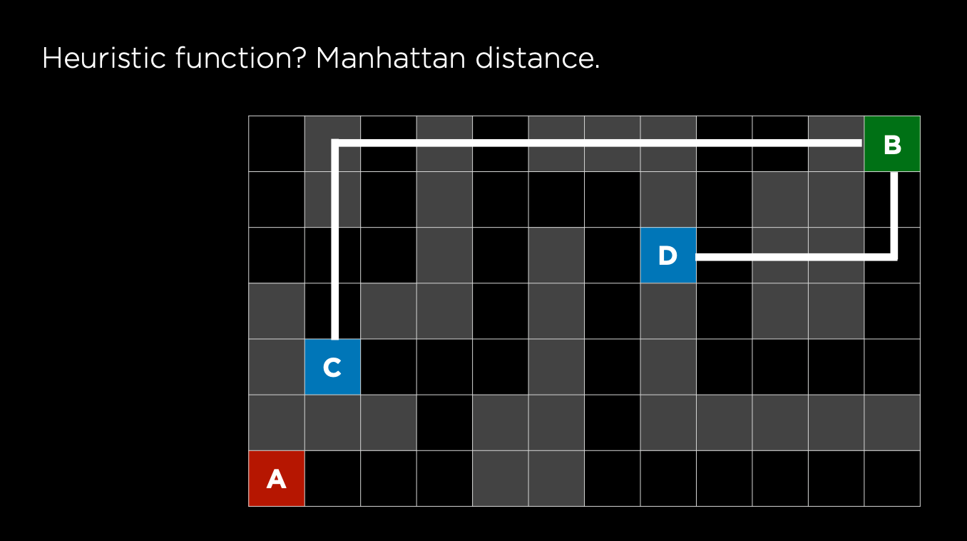
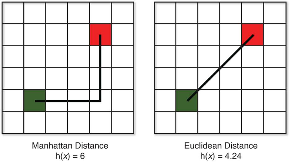
Manhattan distance vs Euclidean distance. We use either of these to estimate the cost from current state to the goal, then choose the action that minimizes the cost
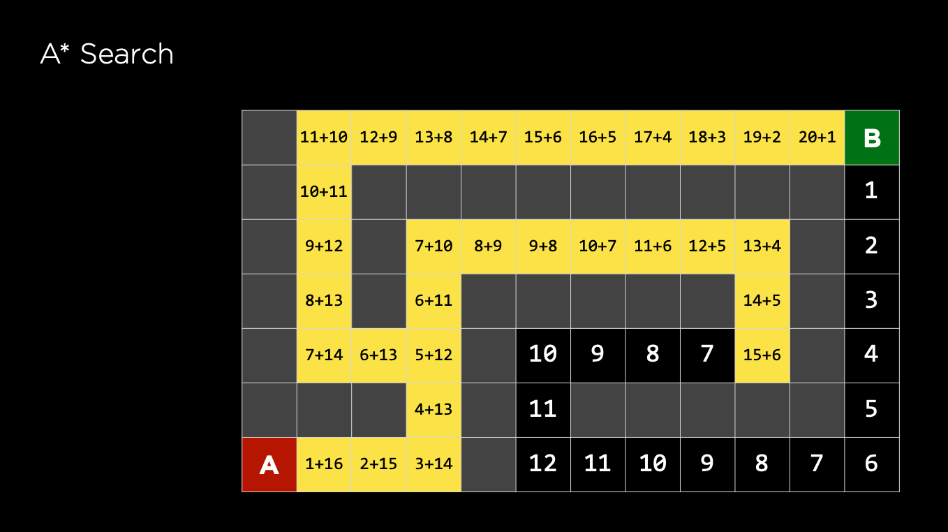
Consider both the cost of path until now and the estimated cost to the goal, g(n) + h(n)
- g(n) = cumalative cost reaching the current node
- h(n) = estimated cost to the destination node
Thus, A* is the best path search algorithm as it considers the distance, weight, cost, etc. and it guarantees to find the shortest path
A* (G, s)  (G is the graph and s is the source node)

    # Order the queue by ascending order of g(n) + h(n)
    let Q be priority_queue
    Q.enqueue( s )
    mark s as visited

    while ( Q is not empty)
        v  =  Q.dequeue( )

        if v is destination then
            return path from s to v

        for all neighbours w of v in Graph G
            if w is not visited
                Q.enqueue( w )
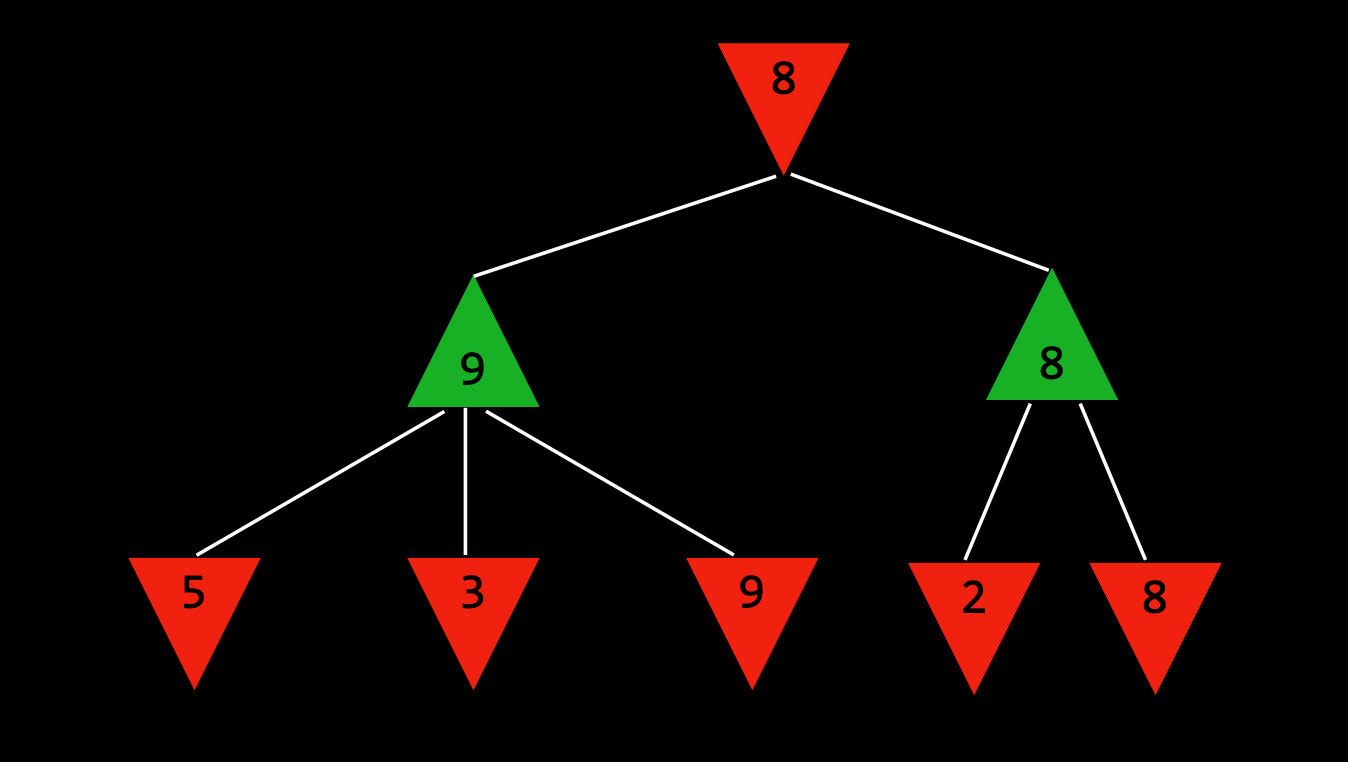
A recursive or backtracking algorithm which is used in decision-making and game theory. It provides an optimal move for the player assuming that opponent is also playing optimally. For instance, in the figure below, the green player is trying to maximize the score and the red player is to minimize to score, which is exactly the same in any game
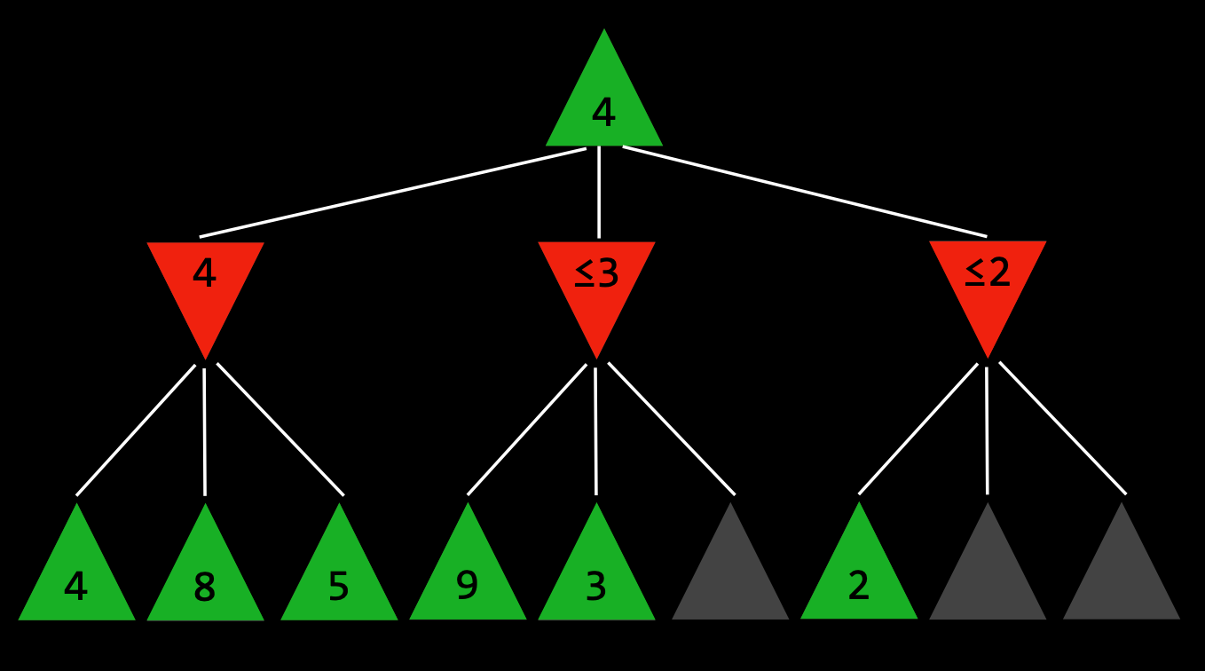
An optimization technique for the Minimax Algorithm
For example, if we want to find the max of three nodes and we know the current node will be definitely less than the previous node, then we do not need to explore every other subnodes of it
A type of Minimax Algorithm that only search to a certain depth, arrive at a decision more quickly
function minimax(node, depth, maximizingPlayer) is
    if depth == 0 or node is a terminal node then
        return static evaluation of node

    if MaximizingPlayer then    // for Maximizer Player
        maxEva= -infinity
        for each child of node do
        eva= minimax(child, depth-1, false)
        maxEva= max(maxEva,eva) //gives Maximum of the values
        return maxEva

    else    // for Minimizer player
        minEva= +infinity
        for each child of node do
        eva= minimax(child, depth-1, true)
        minEva= min(minEva, eva)    //gives minimum of the values
        return minEva
Check out some examples that practice these theories