PNP_final_project_notebook_and_report.jl

### A Pluto.jl notebook ###
# v0.19.11

using Markdown
using InteractiveUtils

# This Pluto notebook uses @bind for interactivity. When running this notebook outside of Pluto, the following 'mock version' of @bind gives bound variables a default value (instead of an error).
macro bind(def, element)
    quote
        local iv = try Base.loaded_modules[Base.PkgId(Base.UUID("6e696c72-6542-2067-7265-42206c756150"), "AbstractPlutoDingetjes")].Bonds.initial_value catch; b -> missing; end
        local el = $(esc(element))
        global $(esc(def)) = Core.applicable(Base.get, el) ? Base.get(el) : iv(el)
        el
    end
end

# ╔═╡ 2eae94d7-4830-4a94-95d4-abbabef7a044
# ╠═╡ show_logs = false
using Printf,PlutoUI,Plots,ExtendableGrids,SimplexGridFactory,VoronoiFVM,GridVisualize,PyPlot ,Triangulate ,LaTeXStrings

# ╔═╡ 470fc128-929b-41fc-b5ce-ff6449ec3111
md"""
# Numerically Solving the One-Dimenional Poisson-Nernst-Planck Equations Using the Finite Volume Method
### Course Project in Scientific Computing at TU Berlin Aditya Kumar and Kay Töpfer
"""

# ╔═╡ 15a44712-fef6-4160-8087-4927b8bbad07
md"""
###
"""

# ╔═╡ aef4afe5-f7b1-4946-9592-42f065b856ce
md"""
## Introduction
"""

# ╔═╡ a0fefd44-853b-4bb9-94fa-8f7bedeacfb1
md"""
 Charge transport is ubiquitous in various applications, such as semiconductors, micro-and-nano-fluidics, and biological ion channels. Charge transportation can be modelled by the Poisson-Nernst-Planck (PNP) equations—a system of coupled nonlinear partial differential equations. The PNP equations describe the diffusion of charged particles (ions) in solution resulting from an electric field, so-called electrodiffusion. The PNP equations can be derived from the gradient flow of an electrostatic free energy, which is based on mean-field approximations of chemical ionic species interactions. Furthermore, the PNP model provides continuum descriptions of chemical species concentration (with the corresponding chemical potential of the species) and the electrostatic potential. 

In the absence of chemical reactions, the two mechanisms that lead to flow of chemical species into or out of a control volume for our problem are diffusion and electromigration—this defines our flux. The electromigration term is defined by coupling the chemical potential generated by the  movement of the charged species concentrations to the applied electrostatic field represented by the Poisson equation. This movement also affects the solute in which the charged species live in, i.e. the neutral solvent. Thus the solvent is transported (migrated) as well. The Nernst-Planck equation is an extension of Fick’s law describing the migration of charged chemical particles in a dilute solution. Fick’s law defines a flux density of species proportional to the gradient of the chemical species concentration and the diffusivity of the species in the neutral solvent. Fick’s law is a macroscopic way of representing the summed effect of the random motion of species owing to thermal fluctuations. As a result, we see that the Nernst-Planck equation forms a continuity equation for the time-dependent species concentration that gives us a conservation law for the underlying physical phenomena of electrodiffusion in dilute solutions. The Poisson and the Nernst-Planck equations together form a system of coupled partial differential equations. Whereas the theory of the Poisson equation is mainly rooted in electrostatics, the Nernst-Planck equation is an incarnation of a conservation law that is only valid for dilute solutions.

The combination of a mean-field approximation ion interactions and continuum theoretic description of chemical properties of the ions provides both quantitative and qualitative  predictions of experimental measurements of chemical species transport problems in many areas of physics and electrical engineering involving semiconductor development, micro-and-nanofluidic device construction, and biologically relevant systems. Although a useful model, there are some limitations. In particular, the number of equations to be solved and the number of diffusion coefficient profiles to be determined for the calculation directly depend on the number of ion species in the system, since each ion species corresponds to one Nernst-Planck equation and one position-dependent diffusion coefficient profile. This leads to the numerical solution of PNP becoming computationally expensive. In this course project, the amount of charged species interacting is two, along with a neutral solvent. Finite-volumes of the charged species and solvent will be taken into account. 

"""

# ╔═╡ 699f7fac-7a4b-4639-b469-d3e721a6baa3
md"""
###
"""

# ╔═╡ 078a97c5-d0f9-4db7-bbe5-127b54c12e2c
md"""
## Setting Up The Problem
As described in the introduction, the Poisson-Nernst-Planck (PNP) equations describe the motions of charged particles that are encountered in various biological, chemical, and physical processes. In a nondimensionalized and simple form, the PNP equations can be written as the following system of coupled nonlinear partial differential equations:

$\begin{align*}
−∇ · ∇φ = q = \sum_{i=1}^{N} z_ic_i \\
\vec J_i = −c_i(∇µ_i + z_i∇φ) \quad (i = 1 . . . N) \\
∂_tc_i + ∇ · \vec J_i = 0 \quad (i = 1 . . . N) \\
\end{align*}$

where the first equation describes the electrostatic potential via the Poisson equation, the second equation describes the flux term, and the third equation is the continuity equation. The second and third equation combined form the Nernst-Planck equation. Altogether we get the Poisson-Nernst-Planck equations. Here, $φ$ is the electrostatic potential, $c_i$ are the species concentrations, and $µ_i$ are the species chemical potentials—the energy necessary to keep a local species configuration. $\vec J_i$ are the species fluxes, $z_i$ the species charge numbers, $q$ is the charge density. The system describes the self-consistent electric field maintained by the charged species, and the species motion due to the electric field $∇φ$ and the gradient of the chemical potential $∇µ_i$. Furthermore, we require that the system be (thermodynamically) closed by establishing a relationship between chemical potential and species concentration. This physical constraint can be codified by the Boltzmann approximation:

$\begin{aligned}
µ_i = log \ c_i \quad (i = 1 . . . N) \\
\end{aligned}$

In electrolytes, a moving species $c_i$ needs to displace the solvent with concentration $c_0$ (and chemical potential µ_0), leading to a modification of the system:

$\begin{aligned}
\vec J_i = −D_ic_i(∇µ_i − ∇µ_0 + z_i∇φ) \quad (i = 1 . . . N)
\end{aligned}$

Once again, we can set $µ_i = log \ c_i$ with $(i = 0 . . . N)$ and add the incompressibility relationship $c_0 + c_1 + · · · + c_N = 1$ that ensures that no concentration can exceed 1. This is physically reasonable as we will have to assume that ions have finite sizes. This relationship allows to express $c_0$ via $c_1 . . . c_N$ and thus to keep just $N$ flux equations. Here the $D_i$ is the diffusion coefficient for each species. The determination of diffusion coefficient for each chemical species would require a combination of extra physical parameters to determine and adjust in order to define the diffusion coefficient. The diffusion coefficient is the amount of a particular substance that diffuses across a unit area in $1$ time step (units usually $1$ second) under the influence of a gradient of one unit. Since the problem is nondimensionalized, we can use the nondimensionalized form of this definition (akin to the notion of "natural units" in some mathematical physics problems) and say that all of the chemical species in our problem have this coefficient set to equal $1$.

For the project we discuss the problem in an $1D$ setting in a domain $Ω = [0, L]$ with $L = 20$. At $x = 0$, we pose the following boundary conditions:

$\begin{align*}
φ = Φ \\
\vec J_i· n = 0 \quad (i = 1 . . . N)
\end{align*}$

For $x = L$, we pose the following boundary conditions: 

$\begin{align*}
φ = 0 \\
c_i = c^∗ \quad (i = 1 . . . N)
\end{align*}$

At $t = 0$ we set the initial conditions $c_i = c^∗$ for $(i = 1 . . . N)$. We look for the simulation in the interval $[0, T]$ with $T = 10^3$ time steps (clarification provided below in "Generate the grid" and "Set values for time evolution"). We assume $N = 2$ and $z_1 = 1$, $z_2 = −1$. Note that for the both the boundary conditions and the initial value, the charge density, $q$, is 0. This situation corresponds to the charging of an ideally polarized electrode, where the positive applied potential
attracts negative ions and repels positive ones, thus creating a double layer with nonzero charge density. With the problem stated, we will now proceed to discuss the finite volume space discretization approach we used for the numerical simulation.
"""

# ╔═╡ 6615b610-6157-4342-b9a0-519e44db5410
md"""
#### Generate the grid

Specifications: 
- 1D
- Domain: $\Omega = [0,20]$
- stepsize = $0.2$
"""

# ╔═╡ acfaaff3-2a03-4e87-a093-c21403b23af3
# ╠═╡ show_logs = false
begin
	# Set domain begin and end
	domain_0 = 0
	domain_L = 20
	grid_step_size = 100
	# Create grid using ExtendableGrids
	grid=ExtendableGrids.simplexgrid(collect(range(domain_0,domain_L,length=grid_step_size+1)))
	# Visulaize grid
	GridVisualize.gridplot(grid,resolution=(600,200),Plotter=PyPlot)
end

# ╔═╡ dd7693a1-0e3d-4b82-8502-fb5b55169615
md"""
#### Set values for time evolution
"""

# ╔═╡ a73b7735-be1c-452c-924a-aa17a3167462
begin
	ini_time = 0
	fin_time = 1000
	dt_step = 1

md"""
Specifications:

- The initial time: ini_time $= 0$
- The final time: fin_time $= 1000$
- The time step increment: dt_step $= 1$
"""

end

# ╔═╡ 2d219416-463d-4def-910b-22a06671f86a
# The Vornoi finite volume method: https://j-fu.github.io/VoronoiFVM.jl/stable/method/

md"""

## Finite Volume Space Discretization of the 1D PNP Equations

The finite volume method has two main ingredients: a geometry based approach to obtain a system describing communicating control volumes and a consistent description of the fluxes between two adjacent control volumes. Rather than reinventing the wheel, we will quote the [VoronoiVFM documentation](https://j-fu.github.io/VoronoiFVM.jl/stable/method/#The-discretization-approach) (which we relied upon heavily) to give a portion of the overview of the finite volume space discretization approach we used. We will further elaborate upon this brief overview. The whole finite volume space discretization of the problem being simulated is thoroughly written below the overview and elaboration.


![](https://j-fu.github.io/VoronoiFVM.jl/stable/vor.png)

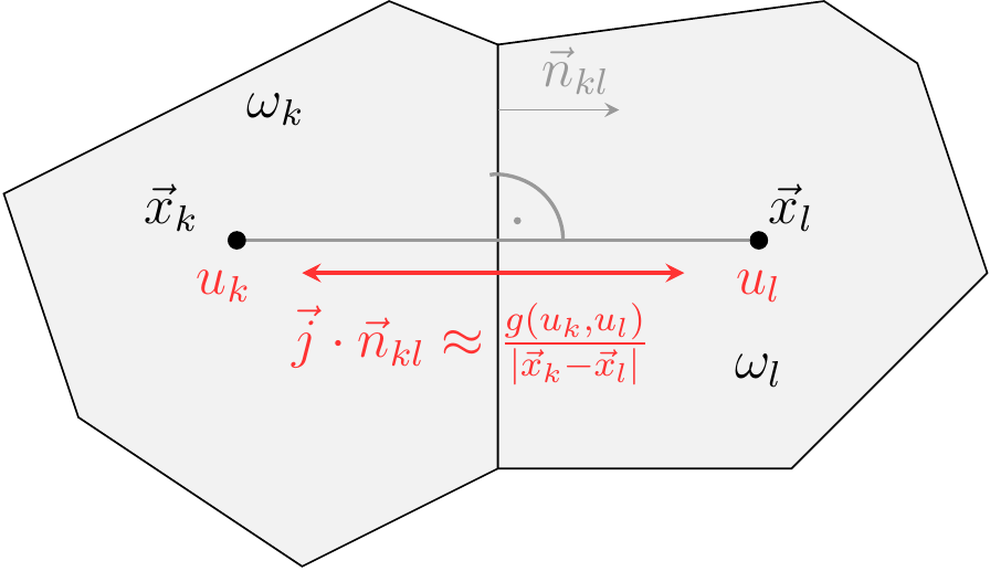
"Given a continuity equation $∇⋅ \vec j=f$ in a domain $Ω$, integrate it over a control volume $\omega_k$ with associated node/collocation point $\vec x_k$, apply Gauss' Divergence Theorem, along with Newton-Leibniz Formula/The Fundamental Theorem of Calculus:

$\begin{aligned}
0&=\int_{\omega_k} (\nabla\cdot  \vec j -f )\ d\omega
=\int_{\partial\omega_k} \vec j\cdot \vec n ds  - \int_{\omega_k} f d\omega\\
&=\sum_{l\in N_k} \int_{\omega_k\cap \omega_l} \vec j\cdot \vec n ds + \int_{\partial\omega_k\cap \partial\Omega} \vec j\cdot \vec n ds   - \int_{\omega_k} f d\omega \\
&\approx \sum_{l\in N_k} \frac{\sigma_{kl}}{h_{kl}}g(u_k, u_l) -  |\omega_k| f_k + \text{boundary terms}
\end{aligned}$

Here, $N_k$ is the set of neighbor control volumes, $\sigma_{kl} = |\omega_k\cap \omega_l|$, $h_{kl}=|\vec x_k - \vec x_l|$, where $|⋅|$ denotes the measure (length resp. area) of a geometrical entity. In the approximation step, we replaced the normal flux integral over the interface between two control volumes by the measure of this interface multiplied by a function depending on the unknowns $u_k$, $u_l$ associated to the respective nodes divided by the distance between these nodes. The flux function  can be derived from usual finite difference formulas discretizing a particular flux law." 

For the boundary terms to be satisfied, we have to implement the various boundary condition types. "To implement a Robin boundary condition on $Γ=∂Ω$:

$- \vec j \cdot \vec n + a u = b,$

we note that by the very construction, the discretization nodes associated to control volumes adjacent to the domain boundary are located at the domain boundary, thus we can assume that the boundary condition is valid in the corresponding collocation node $u_k$. We assume that $\partial\omega_k\cap \partial_\Omega= \cup_{m\in\mathcal M_k} \gamma_{km}$ is the union of a finite number of line (plane) segments. For interior nodes, we set $\mathcal M_k = \emptyset$. Thus, for the boundary terms in the above equation, we have

$\begin{aligned}
\text{boundary terms}&=\sum_{m\in\mathcal M_k} \int_{\gamma_{km}} \vec j \cdot \vec n d s
                     &\approx \sum_{m\in\mathcal M_k} |\gamma_{km}| \vec j \cdot \vec n\\
                     &\approx\sum_{m\in\mathcal M_k} |\gamma_{km}|  (au_k -b),
\end{aligned}$

We observe that for $\varepsilon\to 0$, the Robin boundary condition

$- \vec j \cdot \vec n + \frac{1}{\varepsilon}u = \frac{1}{\varepsilon}g$

tends to the Dirichlet bundary condition

$u=g.$

Therefore, a Dirichlet boundary condition can be approximated by choosing a small value of $\varepsilon$ and implying the aforementioned Robin boundary conditions. This approach called _penalty method_ is chosen for the implementation of Dirichlet boundary conditions in this package.

The entities describing the discrete system can be subdivided into two categories: Geometrical data and Physics-based data. The Geometrical data: $|\omega_k|$, $\gamma_k$, $\sigma_{kl}$, $h_{kl}$ together with the connectivity information simplex grid. These data are calculated from the discretization grid. For the Physics-based data, we have that the number of species and the functions $s$, $g$, $r$, $f$ etc. describing the particular problem. The solution of the nonlinear systems of equations is performed by Newton's method combined with various direct and iterative linear solvers. The Jacobi matrices used in Newton's method are assembled from the constitutive functions whith the help of forward mode automatic differentiation implemented in [ForwardDiff.jl](https://github.com/JuliaDiff/ForwardDiff.jl)" (which uses automatic differentiation via dual numbers and the chain rule).

Now to further elaborate: we want to find some unknowns $u(x,t)$ our solutions that are local species that are stored in $s$, with flux $\vec j$ discretized as $g$, and some reaction term $r$. When we take this type of equations, we can look at them in some representative elementary volume (REV), and apply Gauss' (Ostrogradsky's) Divergence theorem and Newton-Leibniz Rule/Fundamental Theorem of Calculus, in order to make some kind of species balance in this REV. This then gives the change of the amount of species between two moments of time steps that is proportional to what is flowing in or out and to what is created or destroyed during the reaction. This type of view on the problem is very closely linked to the basic physical principles that are used in order to derive these types of systems of partial differential equations (continuity equations/conservational law formulations). Thus, we can discretize such a system by subdividing our domain into artifical REVs (the $\omega_k$ above) with collocation points $\vec x_k$, where we can assign a value of our solution-unknown variable $u$ to certain collocation points associated to each of these REVs. Then we can watch the evolution of these $u$ evaluated at the collocation points due to the integral-balance. Essentially, we get a system of nonlinear equations on the  neighborhood graph of the REV subdivision. Thus, the change of the amount of species during a time interval is proportional to the sum of the fluxes between neighboring REVs and to the amount of species created or destroyed due to the reaction. The time evolution is discretized using implicit Euler for stability purposes. An important point to keep in mind is that the integral formulation of the finite volume method requires that the fluxes are defined as the normal fluxes inside or outside these REVs, along with having the subdivision being formulated in such a way that the interface between two REVs is orthogonal to the two collocation points associated to these two neighboring REVs (also called control volumes). The REV subdivision is generated by first creating boundary conforming Delaunay triangulation of the domain $\Omega$ and then creating a dual Voronoi tessellation where the REVs are now the Voronoi cells.

The finite volume space discretization method has some theoretical advantages: the way this method is derived and formulated essentially exhibits local mass conservation (an important physical property of these systems like the $1D$ PNP); then for convection-diffusion problems, there are robust concepts of upwinding (for discretization of the flux) that allow to avoid, in a guaranteed way (via discrete maximum principle and the M-property of the discretization matrix), unphysical oscillations and we can guarantee positive concentrations in cases where this is important—for the problem of PNP discretization; it can be demonstrated in many cases (in particular for the PNP problem being examined in this project) that there is consistency to thermodynamic principles (a discrete second law of thermodynamics); and finally there are convergence theories for nonlinear systems based on compactness methods.

The flux used in this project is the [SEDAN flux](https://www.wias-berlin.de/preprint/2811/wias_preprints_2811.pdf), which is named after the SEDAN III semiconductor device code. This flux is based on using a discretization approach that is called the Scharfetter-Gummel scheme to approximate the flux at the control volume interface (this is a two-point flux approximation finite volume scheme). This is an exponential fitting upwind flux scheme, which means we have guaranteed sign pattern and M-property. There exist two other variants of fluxes based upon extensions of the Scharfetter-Gummel scheme: the [activity-based flux](https://hal.archives-ouvertes.fr/hal-02194604v3/document) and the [The Bessemoulin-Chatard flux](https://hal.archives-ouvertes.fr/hal-02194604v3/document). Another possible flux discretization approach is the [centered flux](https://www.wias-berlin.de/preprint/2811/wias_preprints_2811.pdf)/[central finite differences](https://www.wias-berlin.de/preprint/2263/wias_preprints_2263_20160708.pdf). This particular approach of using central finite differences for the flux is not used since the scheme may become unstable resulting under certain conditions to large oscillations. Furthermore, the maximum principle can be violated and boundary conditions may be unphysical. 

Aside from other ways of defining the discretized flux for the project, it is also possible to use two other discretization solution methods: finite differences and finite elements. The comparison of these three methods is adequately summarized in [Finite Volume Methods by Robert Eymard, Thierry Gallouët, Raphaèle Herbin](https://hal.archives-ouvertes.fr/hal-02100732v2/document), "From the industrial point of view, the finite volume method is known as a robust and cheap method
for the discretization of conservation laws (by robust, we mean a scheme which behaves well even for particularly difficult equations, such as nonlinear systems of hyperbolic equations and which can easily be extended to more realistic and physical contexts than the classical academic problems). The finite volume method is cheap thanks to short and reliable computational coding for complex problems. It may be more
adequate than the finite difference method (which in particular requires a simple geometry). However, in some cases, it is difficult to design schemes which give enough precision. Indeed, the finite element
method can be much more precise than the finite volume method when using higher order polynomials, but it requires an adequate functional framework which is not always available in industrial problems. Other more precise methods are, for instance, particle methods or spectral methods but these methods can be more expensive and less robust than the finite volume method."

As stated at the beginning of this section on describing the finite volume space discretization approach in general, below is the full finite volume space discretization approach to our problem. We then used VoronoiVFM to implement the discretization and run the numerical simulations.

$\begin{align*}
\\
\\
\\
\partial _x \partial _x \phi - z_1 c_1 - z_2 c_2 &=& 0 \\ 
1-v_0c_0-v_1c_1-v_2c_2 &=& 0 \\
\partial _t c_i +\partial _x [-D_ic_i(\partial _x \log \frac{c_i}{\overline{c}} - \partial _x k_i \frac{c_0}{\overline{c}} + z_i \partial _x \phi)] &=& 0 \\
\\
\end{align*}$

Flux terms:

$\begin{align*}
J_{\phi} &=& \partial _x \phi \\
J_{c_0} &=& 0 \\
J_{c_1} &=& -D_1c_1(\partial _x \log \frac{c_1}{\overline{c}} - \partial _x k_1 \frac{c_0}{\overline{c}} + z_1 \partial _x \phi) \\
J_{c_2} &=& -D_2c_2(\partial _x \log \frac{c_2}{\overline{c}} - \partial _x k_2 \frac{c_0}{\overline{c}} + z_2 \partial _x \phi) \\
\end{align*}$

Reaction terms:

$\begin{align*}
R_{\phi} &=& - z_1 c_1 - z_2 c_2 \\
R_{c_0} &=& 1-v_0c_0-v_1c_1-v_2c_2 \\
R_{c_1} &=& 0 \\
R_{c_2} &=& 0
\end{align*}$

---

From $J_{c_{1/2}}$ to $g_{c_{1/2}}$:

$J_{c_{1/2}} = -D_ic_i(\partial _x \log \frac{c_i}{\overline{c}} - \partial _x k_i \frac{c_0}{\overline{c}} + z_i \partial _x \phi)$ 

Desired form:

$J_{des} = -D_i(\partial _x c_i - c_i \frac{v}{D_i})$

Since $\partial _x \log c_i = \frac{1}{c_i} \cdot \partial _x c_i$:

$J_{c_{1/2}} = -D_i [\partial _x c_i - c_i (k_i \partial _x \log(c_0) - (k_i-1)\log(\overline{c}) - z_i \partial _x \phi)]$

$v = D_i [k_i \partial _x \log(c_0) - (k_i-1)\log(\overline{c}) - z_i \partial _x \phi]$

$v_{kl} = \frac{D_i}{|\sigma|} \cdot[k_i \int _{\sigma} \partial _x \log(c_0) d \gamma - (k_i-1) \int _{\sigma} \partial _x \log(\overline{c}) d \gamma -  z_i \int _{\sigma} \partial _x \phi d \gamma]$
$v_{kl} = \frac{D_i}{h_{kl}} [k_i \log(\frac{c_{0_R}}{c_{0_L}}) + (k_i-1) \log(\frac{\overline{c}_L}{\overline{c}_R})+ z_i (\phi _L - \phi _R)]$

$g_{c_{1/2}} = D_i(B(\frac{v_{kl}h_{kl}}{D_i})c_L - B(\frac{-v_{kl}h_{kl}}{D_i})c_R)$

---
Applied BC

$\phi (0) = \frac{1}{2}$
$\phi (L) = 0$
$c_i(L) = \frac{1}{3}$
$J_i \cdot n = 0$

---
Applied IC

$\phi = \frac{1}{2}$
$c_i = \frac{1}{3}$

---

Defined Variables

$D_i = 1$
$z_0 = 0$
$z_1 = -1$ 
$z_2 = 1$
$v_0 = 1$
$v_1 = 1$
$v_2 = 1$

---

Other Variables (for clearification)

$\begin{align*}
\overline{c} &=& \sum c_i \\
k_i &=& \frac{v_i}{v_0} = const. \\
\end{align*}$
$\newline$

"""

# ╔═╡ 0e996cc2-ce10-44ce-8698-bc77ee0819e4
md"""
## VoronoiFVM Implementation of FVM Discretization of 1D PNP Equations
"""

# ╔═╡ 2c0b8207-5f12-424d-81b8-d4adb2c202c7
begin

# Create the mutable struct "Data" which is able to hold all the needed variables
mutable struct Data
    z_1::Float64
	z_2::Float64
	D::Float64
	v_0::Float64
	v_1::Float64
	v_2::Float64
	k_1::Float64
	k_2::Float64
	ic0::Int32
    ic1::Int32
	ic2::Int32
    iphi::Int32
    Data()=new()
end

# Set which species are under time derivate
function storage!(f,u,node,data)
	
	# Import values from data
	ic0 = data.ic0
    ic1 = data.ic1
	ic2 = data.ic2	
    iphi = data.iphi
	
	# c_1 and c_2 are time derivable ones
    f[iphi] = 0 
	f[ic0] = 0 
    f[ic1] = u[ic1]
	f[ic2] = u[ic2]
end

# Set reaction terms 	
function reaction!(f,u,node,data)
	
	# Import values from data
	ic0 = data.ic0	
    ic1 = data.ic1
	ic2 = data.ic2
    iphi = data.iphi
	z_1 = data.z_1
	z_2 = data.z_2
	v_0 = data.v_0
	v_1 = data.v_1
	v_2 = data.v_2
	
	# Reaction terms	
    f[iphi] = -(z_1*u[ic1]+z_2*u[ic2])
	f[ic0] = 1 - v_0*u[ic0] - v_1*u[ic1] - v_2*u[ic2]
    f[ic1] = 0
	f[ic2] = 0
end

# Set flux terms
function sedanflux!(f,u0,edge,data)
    u=unknowns(edge,u0)
	
	# Import values from data
	ic0 = data.ic0
    ic1 = data.ic1
	ic2 = data.ic2
    iphi = data.iphi
	D = data.D
	z_1 = data.z_1
	z_2 = data.z_2
	k_1 = data.k_1
	k_2 = data.k_2

	# Calculate the logarithmns needed for the flux terms
	log_min = -5
	log_res_c0 = log(abs(u[ic0,2]/u[ic0,1]))
	log_res_c012 = log(abs((u[ic0,1]+u[ic1,1]+u[ic2,1])/(u[ic0,2]+u[ic1,2]+u[ic2,2])))

	# If the logarithms smaller than log_min, set the logarithms to log_min to avoid errors caused by high negativ logarithmns
	if log_res_c0 < log_min
		log_res_c0 = log_min
	end
	if log_res_c012 < log_min
		log_res_c012 = log_min
	end

	# Flux terms
    f[iphi] = u[iphi,1]-u[iphi,2]
	f[ic0] = 0
	bp1, bm1 = fbernoulli_pm(k_1*log_res_c0+(k_1-1)*log_res_c012+z_1*(u[iphi,1]-u[iphi,2])) # bernoulli function
	bp2, bm2 = fbernoulli_pm(k_2*log_res_c0+(k_2-1)*log_res_c012+z_2*(u[iphi,1]-u[iphi,2])) # bernoulli function
	f[ic1] = D*(bm1*u[ic1, 1]-bp1*u[ic1, 2]) 
	f[ic2] = D*(bm2*u[ic2, 1]-bp2*u[ic2, 2]) 
end

# Main function to solve the problem
function main_problem(;n=20,Plotter=nothing,dlcap=false,verbose=false,unknown_storage=:sparse,DiffEq=nothing, t_min, t_max, t_step, t_step_max, c1_dir, c2_dir, v_0, v_1, v_2)
	
	# Specify h and grid
    h=20/convert(Float64,n)
    grid=VoronoiFVM.Grid(collect(0:h:20))

	# Save needed variables in data
    data = Data()
    data.z_1 = -1
	data.z_2 = 1
	data.D = 1
	data.v_0 = v_0
	data.v_1 = v_1
	data.v_2 = v_2
	## Species number
    data.iphi = 1
    data.ic1 = 2
	data.ic2 = 3
	data.ic0 = 4

	# Import values from data
	ic1 = data.ic1
	ic2 = data.ic2
    iphi= data.iphi
	ic0 = data.ic0
	v_0 = data.v_0
	v_1 = data.v_1
	v_2	= data.v_2

	# Calculate k_1 and k_2 and save it in data
	data.k_1 = v_1 / v_0
	data.k_2 = v_2 / v_0

	# Set up the physics
    physics=VoronoiFVM.Physics(data=data,
                               num_species=4,
                               flux=sedanflux!,
                               reaction=reaction!,
                               storage=storage!
                               )

	# Create finite volume system
    sys=VoronoiFVM.System(grid,physics,unknown_storage=unknown_storage)

	# Enable species
    enable_species!(sys,1,[1])
    enable_species!(sys,2,[1])
	enable_species!(sys,3,[1])
	enable_species!(sys,4,[1])

	# Set boundary conditions
	## Dirichlet
    boundary_dirichlet!(sys,iphi,1,0.5)
    boundary_dirichlet!(sys,iphi,2,0.0)
	boundary_dirichlet!(sys,ic0,2,1-c1_dir-c2_dir)
    boundary_dirichlet!(sys,ic1,2,c1_dir)
	boundary_dirichlet!(sys,ic2,2,c2_dir)	
	# Neumann
	boundary_neumann!(sys,ic0,1,0)
	boundary_neumann!(sys,ic1,1,0)
	boundary_neumann!(sys,ic2,1,0)

	# Set initial conditions
    inival=unknowns(sys)
    @views inival[iphi,:].=0.5
	@views inival[ic0,:].=1-c1_dir-c2_dir
    @views inival[ic1,:].=c1_dir
	@views inival[ic2,:].=c2_dir


	# Solve the system
    ## Create solver control info for constant time step size
    control=VoronoiFVM.NewtonControl()
    control.verbose=verbose
    control.Δt_min=0
    control.Δt=t_step
    control.Δt_grow=1.2
    control.Δt_max=t_step_max
    control.Δu_opt=100
    control.damp_initial=0.5
    if isnothing(DiffEq)
        tsol=solve(inival,sys,[t_min,t_max],control=control)
    else 
        tsol=solve(DiffEq,inival,sys,[0.0,10],
                   initializealg=DiffEq.NoInit(),
                   dt=t_step)	
    end

	# Return solution
	return tsol
end
end

# ╔═╡ 0d1ac969-ce6a-45c6-9c7e-3675cc858055
md"""
### Calculate Solution
"""

# ╔═╡ cb94ba74-a654-4ccd-bfd0-7309e3899c21
# ╠═╡ show_logs = false
solution = main_problem(;n=grid_step_size,Plotter=PyPlot,dlcap=true,verbose=true,unknown_storage=:sparse,DiffEq=nothing, t_min=ini_time, t_max=fin_time, t_step=dt_step, t_step_max=0.1, c1_dir=1/3, c2_dir=1/3, v_0=1, v_1=1, v_2=1);

# ╔═╡ fdf88786-5691-422c-9484-fa905c47bcde
md"""
#
"""

# ╔═╡ d4ea8aa9-cec8-4cfa-8ed3-22a32f0c0fdc
md"""
## Presentation of Results
"""

# ╔═╡ 95ecd8a5-8d5f-48ef-a4c4-b4eb1ac131c5
# Define some functions to make plotting easier
begin
	# Create visualizer and set x limit
	visualizer=GridVisualizer(Plotter=PyPlot, resolution=(700,700),layout=(2,1), xlimits=(domain_0, domain_L))

	# Function for plotting our scalar plots
	function scalarPlots(solution, num_species, time_var)
		t = round(solution.t[time_var]*100)/100
		scalarplot!(visualizer[1,1],grid,solution[:,time_var][1,:],title="Potential at time t=$t",flimits=(minimum(solution),maximum(solution)*1.05), xlabel = latexstring("Domain  \$\\Omega\$"), ylabel = latexstring("Potential  \$\\Phi\$"))
	
		scalarplot!(visualizer[2,1],grid,solution[:,time_var][2,:],title="Concentrations at time t=$t",flimits=(0,1),color=:blue,label="\$c_1\$", xlabel = latexstring("Domain  \$\\Omega\$"), ylabel = latexstring("Concentration  \$c\$"), legend=:best)
	
		scalarplot!(visualizer[2,1],grid,solution[:,time_var][3,:],flimits=(0,1),color=:red,clear=false,label="\$c_2\$", xlabel = latexstring("Domain  \$\\Omega\$"), ylabel = latexstring("Concentration  \$c\$"))

		if num_species == 4
			scalarplot!(visualizer[2,1],grid,solution[:,time_var][4,:],flimits=(0,1),color=:green,clear=false,label="\$c_0\$", xlabel = latexstring("Domain  \$\\Omega\$"), ylabel = latexstring("Concentration  \$c\$"))
		end
		reveal(visualizer)

	end

	# Function to get the arrays needed for our contour plots
	function contourArrays(input_array, num_species, grid_len)
		time_len = length(input_array)
		output_dict = Dict() 
		for i in 1:num_species
			temp_array = input_array[:,1][i,:] # temporary array for cache
			for j in 2:time_len
				append!(temp_array, input_array[:,j][i,:])
			end
			output_dict[i] = temp_array
		end
		return output_dict, time_len
	end

	# Function for plotting the countor plots
	function contourPlots(contour_dict, num_species, time_len, c_max, automatic_lims)
		x = grid[Coordinates][:]
		y = log10.(1:time_len)
		plot_dict = Dict()

		if automatic_lims == true
			clims_phi = :auto
			clims_c = :auto
		else
			clims_phi = (0,0.5)
			clims_c = (0,c_max)
		end
		plot_dict[1] = Plots.contour(x, y, contour_dict[1], fill = true, title=latexstring("Potential \$\\phi\$"), xlabel = latexstring("Domain  \$\\Omega\$"), ylabel = latexstring("timestep in \$10^x\$"), linewidth = 0, c = :redsblues, clims=clims_phi)
		plot_dict[2] = Plots.contour(x, y, contour_dict[2], fill = true, title=latexstring("Concentration \$c_1\$"), xlabel = latexstring("Domain  \$\\Omega\$"), ylabel = latexstring("timestep in \$10^x\$"), linewidth = 0, c = :roma, clims=clims_c)
		plot_dict[3] = Plots.contour(x, y, contour_dict[3], fill = true, title=latexstring("Concentration \$c_2\$"), xlabel = latexstring("Domain  \$\\Omega\$"), ylabel = latexstring("timestep in \$10^x\$"), linewidth = 0, c = :roma, clims=clims_c)
		if num_species == 4
			plot_dict[4] = Plots.contour(x, y, contour_dict[4], fill = true, title=latexstring("Concentration \$c_0\$"), xlabel = latexstring("Domain  \$\\Omega\$"), ylabel = latexstring("timestep in \$10^x\$"), linewidth = 0, c = :roma, clims=clims_c)
		end
		return plot_dict
	end

	# Function for plotting our animations
	function animations(solution, num_species, animation_step)
		x = grid[Coordinates][:]
		min_sol = round(minimum(solution))
		max_sol = round(maximum(solution))
		time_len = length(solution)
		
		
		anim_solution = @animate for i = 1:animation_step:time_len
			Plots.contour(x, min_sol:max_sol, append!(solution[:,i][1,:], solution[:,i][1,:]), fill = true, ticks = true, linewidth = 0, c = :redsblues, clims=(0,0.5), title="Potential and Concentrations over time", colorbar_title="Potential \$\\phi\$")
		
			Plots.plot!(x, solution[:,i][2,:], ylims = (min_sol, max_sol), xlims = (domain_0, domain_L), linewidth=3, linecolor="aqua", xlabel = latexstring("Domain  \$\\Omega\$"), ylabel = latexstring("Concentration \$c\$"), label="\$c_1\$")
		
			Plots.plot!(x, solution[:,i][3,:], linewidth=3, linecolor="fuchsia", label="\$c_2\$")

			if num_species == 4
				Plots.plot!(x, solution[:,i][4,:], linewidth=3, linecolor="green", label="\$c_0\$")
			end
		end
		return anim_solution
	end
	
end

# ╔═╡ bfebf9f5-57a1-4d2d-b010-31c33f28c5d5
md"""
### Scalar Plots of Species Concentrations and Potential
#### Slider for time t
"""

# ╔═╡ a2e9f3cb-93bf-4e8d-82a4-bed79423a6ea
@bind time Slider(1:1:length(solution))

# ╔═╡ 23b59e41-c5a8-4de6-882c-019a87d74fef
println("t = "*string(round(solution.t[time]*100)/100))

# ╔═╡ 4ff1af93-59a7-4d0b-b19e-e85d216e4398
scalarPlots(solution, 4, time)

# ╔═╡ cb43d58e-454c-4e65-afe2-f14e876f127a
md"""
"""

# ╔═╡ 6e9cc937-bfde-4aa7-9615-fbb1a45bd0d1
md"""
### Contour Plots of the Time Evolution of Concentrations and Potential
"""

# ╔═╡ a06a6592-4206-41eb-b18f-8a5fa3dd87e8
begin
	contour_dict, time_len = contourArrays(solution, 4, grid_step_size + 1)
	contour_plots = contourPlots(contour_dict, 4, time_len, 0.5, false)

	Plots.plot(contour_plots[2], contour_plots[3])
end

# ╔═╡ b282a67c-799e-406a-97c9-9f8952133c02
Plots.plot(contour_plots[4], contour_plots[1])

# ╔═╡ 914bbe12-14b2-461e-b678-be84e014c40e
md"""
### 
"""

# ╔═╡ 69f6fd9b-8a37-46e4-a1cb-94f3d53cc841
md"""
### Animation of the Above Scalar and Contour Plots Combined
"""

# ╔═╡ c4c34aaa-c15a-478e-b86a-0479c3b0dcbf
# ╠═╡ show_logs = false
begin
	animated_solution = animations(solution, 4, 10)
	gif(animated_solution, "animated_solution.gif", fps = 30)
end

# ╔═╡ 62fdd60b-b26d-4802-91df-aea028296e85
md"""
####
"""

# ╔═╡ 82157790-e629-44b8-864d-09fbb61aa484
md"""
The plots and animations above show that the evolution of potential $\phi$, concentration of negative ($c_1$), positive ($c_2$) and solvent ($c_0$). Both the two charged species and the solvent have equal size/volume $v_0=v_1=v_2=1)$. The results show the following: there is an attraction of the negative charged species ($c_1$) to $x=0$ because $\phi$ at $x=0$ is larger than $\phi$ at $x=L$; and there is a repelling of the positive charged species ($c_2$) from $x=0$ because $\phi$ at $x=0$ is larger than $\phi$ at $x=L$. This leads to the results exhibiting double layer charging. Furthermore, the results show that at $x=L, c_i=c^*=1/3$ for $\ i=0,1,2$, we have that all of the species have the same concentration on the right side of the domain, i.e. $+\phi(x=0)=\phi _0 = 1/2$ and  $\phi(x=L) = \phi _L = 0$. This shows that the dirichlet boundary conditions are fullfilled.

It almost makes sense physically—the positive species concentration increases by a marginal amount, and the incompressibility condition though satisfied ends up decreasing the solvent concentration, which affects the mass conservation—solvent concentration should not have decreased. The positive species concentration increased due to the collision flux at the boundary layer where the applied positive potential is located. As soon as the positive chemical species arrives at this boundary, the self-consistent field condition of the Poisson equation of the applied electric potential creates a sort-of-feedback with the positive charges of the chemical species. As stated above, at $x=0$ we have a double layer charging occuring at this boundary where there is an applied electrostatic potential.

This is almost physically reasonable, although not quite correct dynamics of the physical system, but there seems to be an issue with the conservation of concentration of our two species, $c_1$ and $c_2$, and our solvent $c_0$. The concentrations are all positive and conserved. From the graph in our code, it looks like there is a small creation of species concentration for $c_1$ as that particular species diffuses towards our "source" of the initial electric potential on the left-hand boundary at $x = 0$. Because of the self-consistent field approach to our system, the sudden creation of more species concentration around $x = 0$ is due to the reliance of the distribution of charges creating the electric field and the electric field relying upon the distribution of charges—seeing the attraction/repelling of species according to their charge around the boundary layer. This is an almost-physically-correct solution given that there is a slight issue with the rising of concentration values for our species $c_1$ and $c_2$, which is not physically correct but, it can be interpreted as physically correct by observing the self-consistent field approach and the way we set up the "reaction" terms for our discretization within the Voronoi API.
"""

# ╔═╡ 96b27dfd-b4a6-4531-bf55-a4ed717467c2
md"""
###
"""

# ╔═╡ 69df9d73-3733-4b1f-92da-a7cf2622a71e


# ╔═╡ f4675a1a-a6b9-4306-91ba-a0d6710c5afd
md"""
### Plots for Different Ion Volume



$v_1 = 2$ 
$v_2 = 1$ 
$v_0 = 1$

"""

# ╔═╡ 1056ab3e-edae-486c-bdcc-84c8c9765abb
# ╠═╡ show_logs = false
solution_diff_vol = main_problem(;n=grid_step_size,Plotter=PyPlot,dlcap=true,verbose=true,unknown_storage=:sparse,DiffEq=nothing, t_min=ini_time, t_max=fin_time, t_step=dt_step, t_step_max=0.1, c1_dir=1/3, c2_dir=1/3, v_0=1, v_1=1.5, v_2=1);

# ╔═╡ 971fc5e4-ce3c-4c39-a7cf-f4e35e2f8c63
begin
	contour_dict_diff_vol, time_len_diff_vol = contourArrays(solution_diff_vol, 4, grid_step_size + 1)
	contour_plots_diff_vol = contourPlots(contour_dict_diff_vol, 4, time_len_diff_vol, 0.5, false)

	Plots.plot(contour_plots_diff_vol[2], contour_plots_diff_vol[3])
end

# ╔═╡ 582814b0-0410-4356-82b3-845fef6e7978
Plots.plot(contour_plots_diff_vol[4], contour_plots_diff_vol[1])

# ╔═╡ 5b283a49-510b-4d9e-b29d-7dd41d0bf3eb
md"""
The plots above involving the finite volume show the evolution of potential $\phi$, the concentrations of the negative ($c_1$), the positive ($c_2$), and the solvent ($c_0$) charged species with volumne of ions for $c_0, c_1,$ and $c_2$ given by $v_0=v_2 = 1$ and $v_1=2$. The volume of the negative charged species is double that of the volume of the positive charged species and the solvent. There is an attraction of the negative charged species ($c_1$) to the $x=0$ boundary due to the positive $\phi$ at $x=0$ being larger than $\phi$ at $x=L$. There is a repelling of the positive charged species ($c_2$) from $x=0$ because $\phi$ at $x=0$ is larger than  $\phi$ at $x=L$. This leads to the observation of the double layer charging phenomena. Furthermore, the concentrations of both the negative charged species and the solvent are lower at $x=0$. The concentration of negative charged species is lower in the rest of the domain (but at $x=L$, $c_1=1/3$ for $v_1=1$ and $v_1=2$). The results also show that the concentration of positive charged species is a bit higher over the domain (but at $x=L$, $c_2=1/3$ for $v_1=1$ and $v_1=2$). This is because of similar reasons stated in the previous section on the interpretation and presentation of the plots and animations of the concentrations are all initially equal and the sizes/volumes of species and solvent are all equal.
"""

# ╔═╡ 3ff2cc4c-81a6-4484-a3a0-a0c1916cddf1
md"""
###
"""

# ╔═╡ 6dc1afff-12f4-4f22-a60c-5ba843facadd


# ╔═╡ ef9ce3be-f0bc-4cd9-931e-cfdd0cc559c2
md"""
### Results for Varying Values of $c^*$ for $c_1$ and $c_2$
"""

# ╔═╡ de92b301-eaec-4b10-8a3b-454c6393ef9e
md"""
##### Set values for stepsize, the smallest and the largest possible $c^*$
"""

# ╔═╡ bae36b4f-90d7-41a9-ba30-5607a085fa62
begin
	c_start = 0.05
	c_step = 0.05
	c_end = 0.95

	md"""
	Specifications:
	
	$c_{start} = 0.05$
	$c_{step} = 0.05$
	$c_{end} = 0.95$
	"""
end

# ╔═╡ a37133fc-0f30-409a-a4aa-57e3de882963
# ╠═╡ show_logs = false
begin
	# Going through every combination of c_1 and c_2
	begin
		global solution_array_c1_c2 = [] 
		for c2_dir in c_start:c_step:c_end # go through every possibility for c_2
			global solution_array_c1 = []
			for c1_dir in c_start:c_step:c_end # gp through every possibility for c_1
				try # try to get a solution for each combination
	    			global solution_combination = main_problem(;n=grid_step_size,Plotter=PyPlot,dlcap=true,verbose=true,unknown_storage=:sparse,DiffEq=nothing, t_min=ini_time, t_max=1000, t_step=1, t_step_max=10, c1_dir, c2_dir, v_0=1, v_1=1, v_2=1)
				catch combination_doesnt_work
					global solution_combination = [0]
				end
				push!(solution_array_c1, solution_combination)
			end
			push!(solution_array_c1_c2, solution_array_c1) # save every combination in solution_array_c1_c2
		end
	end
	
	md"""
	In order to show the results for diffrent combinations of $c_1$ and $c_2$, the results for every combination of $c_1$ and $c_2$ were calculated.
	"""
end

# ╔═╡ cee4bd55-1861-4efc-bf04-79521a6803de
md"""
#### Slider for $c_1$ and $c_2$
"""

# ╔═╡ 9848decf-5fca-4fc4-bef4-77463778e6cf
@bind c1_pos Slider(1:1:length(solution_array_c1))

# ╔═╡ 338930f9-0d99-48ec-803a-e4eeb2dac207
c_1 = round((c_start+(c1_pos-1)*c_step)*100)/100

# ╔═╡ d6841195-f4df-46c1-bfa3-2be5c2d54e77
@bind c2_pos Slider(1:1:length(solution_array_c1))

# ╔═╡ b6dc67de-9ba6-4301-93ef-6c88823f5269
c_2 = round((c_start+(c2_pos-1)*c_step)*100)/100

# ╔═╡ f85ed8b7-fede-4458-9e1a-0e2510a932b0
md"""
### Contour plots of the Time Evolution of Varying $c_1$ and $c_2$
"""

# ╔═╡ 25993f86-3457-49b8-bf21-9573a86471d7
begin
	try
		contour_dict_c1_c2, time_len_c1_c2 = contourArrays(solution_array_c1_c2[c2_pos][c1_pos], 4, grid_step_size + 1)
		global contour_plots_c1_c2 = contourPlots(contour_dict_c1_c2, 4, time_len_c1_c2, max(c_1,c_2,1-c_1-c_2), true)
		Plots.plot(contour_plots_c1_c2[2], contour_plots_c1_c2[3])
	catch
		println("Combination does not work")
	end
end

# ╔═╡ 228a62af-47c3-485e-adde-d59e980e426f
begin
	try
		Plots.plot(contour_plots_c1_c2[4], contour_plots_c1_c2[1])
	catch
		println("Combination does not work")
	end
end

# ╔═╡ e9198ceb-479b-4b95-93a8-6f3c1beb3c43
md"""
The above plots show the following: 

When reducing the concentration of the positive charged species $c_2$ (in comparison to the case in the previous section above), it is observed that at end of time evolution $\phi$ at $x$ is larger than $\phi$ at $x=L$, which is $0$ for most part of the interior of the domain. The concentration of the positive charged species is low on both sides of the domain than in the case above in the previous section. The concentration of the negative charged species is higher at $c_1$ at $x=0$ than at $c_1$ at $x=L$. The concentration of the solvent is, in general (across the domain), higher throughout the evolution.

When increasing the concentration of the positive charged species $c_2$ (in comparison to the case in the previous section above), it is observed that at the end of the time evolution $\phi$ at $x$ is larger than $\phi$ at $x=L$, which is $0$ for all $x \in \Omega$. Results also show that $c_2$ at $x=0$ is smaller than $c_2$ at $x=L$ and $c_1$ at $x=0$ is larger than $c_1$ at $x=L$. The concentration of the solvent is, in general (across the domain), lower throughout the evolution.

When reducing the concentration of the negative charged species $c_1$ (in comparison to the case above), it is observed that at the end of the time evolution $\phi$ at $x$ is larger than $\phi$ at $x=L$, which is equal to $0$ for all $x \in \Omega$. Furthermore, the following is observed: $c_2$ at $x=0$ is smaller than $c_2$ at $x=L$; $c_1$ at $x=0$ is larger than $c_1$ at $x=L$; and the concentration of the solvent is, in general (across the domain), higher throughout the evolution.

When increasing the concentration of the negative charged species $c_1$ (in comparison to the case above), it can be seen that at the end of the time evolution
$\phi$ at $x$ is larger than $\phi$ at $x=L$, which is equal to $0$ for most of the interior of the domain. Furthermore, the following observations can be made: $c_2$ at $x=0$ is smaller than $c_2$ at $x=L$; the concentration of the negative charged species is higher on both the domain and the boundaries relative to the case above; $c_1$ at $x=0$ is larger than $c_1$ at $x=L$; and finally the concentration of the solvent is, in general (across the domain), lower throughout the evolution

Finally, it is observed that some combinations of concentrations are not feasible. This could be due to the combination of the incompressibility condition being imposed and the issues discussed in the first results section documenting the issues with concentration conservation and the applied electrostatic potential building a double layer that may be affecting the species concentration due to the self-consistent field.

"""

# ╔═╡ a3192f15-7ac5-485e-9a32-556226f1faa0


# ╔═╡ 6d70eea9-7ff9-4803-8c04-bf8b7b8301cc
md"""
# Simplification of Original Problem by Removal of Solvent $c_0$ 
"""

# ╔═╡ 070a943f-3e50-4c9b-bd55-d91ae124f85a
md"""
## Finite Volume Space Discretization of the Simplied 1D PNP Equations (removal of $c_0$)
We remove the solvent from the original 1D PNP equations in order to compare this simplification to the original 1D PNP equations above. By removing the solvent term, we have a simplified two chemical species system with the corresponding incompressibility condition and volume condition. The reaction and flux terms are defined below.

$\begin{align*}
\partial _x \partial _x \phi - z_1 c_1 - z_2 c_2 &=& 0 \\ 
1-v_1c_1-v_2c_2 &=& 0 \\
\partial _t c_i +\partial _x [-D_ic_i(\partial _x \log \frac{c_i}{\overline{c}} + z_i \partial _x \phi)] &=& 0 \\
\\
\end{align*}$

Flux terms:

$\begin{align*}
J_{\phi} &=& \partial _x \phi \\
J_{c_1} &=& -D_1c_1(\partial _x \log \frac{c_1}{\overline{c}} + z_1 \partial _x \phi) \\
J_{c_2} &=& 0 \\
\end{align*}$

Reaction terms:

$\begin{align*}
R_{\phi} &=& - z_1 c_1 - z_2 c_2 \\
R_{c_1} &=& 0 \\
R_{c_2} &=& 1-v_1c_1-v_2c_2 \\
\end{align*}$

---

From $J_{c_{1/2}}$ to $g_{c_{1/2}}$:

$J_{c_{1}} = -D_1c_1(\partial _x \log \frac{c_1}{\overline{c}} + z_1 \partial _x \phi)$ 

Desired form:

$J_{des} = -D_1(\partial _x c_1 - c_1 \frac{v}{D_1})$

Since $\partial _x \log c_1 = \frac{1}{c_1} \cdot \partial _x c_1$:

$J_{c_{1}} = -D_1 [\partial _x c_1 - c_1 (\log(\overline{c}) - z_1 \partial _x \phi)]$

$v = D_1 [\log(\overline{c}) - z_1 \partial _x \phi]$

$v_{kl} = \frac{D_1}{|\sigma|} \cdot[\int _{\sigma} \partial _x \log(\overline{c}) d \gamma -  z_1 \int _{\sigma} \partial _x \phi d \gamma]$

$v_{kl} = \frac{D_1}{h_{kl}} [\log(\frac{\overline{c}_R}{\overline{c}_L})+ z_1 (\phi _L - \phi _R)]$

$g_{c_{1}} = D_i(B(\frac{v_{kl}h_{kl}}{D_1})c_L - B(\frac{-v_{kl}h_{kl}}{D_1})c_R)$

---
Applied BC

$\phi (0) = \frac{1}{2}$
$\phi (L) = 0$
$c_i(L) = \frac{1}{2}$
$J_i \cdot n = 0$

---
Applied IC

$\phi = \frac{1}{2}$
$c_i = \frac{1}{2}$

---

Defined Variables

$D_i = 1$
$z_1 = -1$ 
$z_2 = 1$
$v_1 = 1$
$v_2 = 1$

---

Other Variables (for clearification)

$\begin{align*}
\overline{c} &=& \sum c_i = c_1 + c_2 \\
\end{align*}$
$\newline$

"""

# ╔═╡ 675092ef-b725-4c00-ba0d-26b82ac4735c
md"""
## VoronoiFVM Implementation of FVM Discretization of the Simplified 1D PNP Equations
"""

# ╔═╡ 3aa234a5-2058-4715-af9b-f2a1d4bca2b4
# Works like above - but diffrent reaction & flux terms

begin

function storage_reduced!(f,u,node,data)
    ic1 = data.ic1
	ic2 = data.ic2	
    iphi = data.iphi
    f[iphi] = 0 
    f[ic1] = u[ic1]
	f[ic2] = 0
end

function reaction_reduced!(f,u,node,data)
    ic1 = data.ic1
	ic2 = data.ic2
    iphi = data.iphi
	z_1 = data.z_1
	z_2 = data.z_2
	v_1 = data.v_1
	v_2 = data.v_2
		
    f[iphi] = -(z_1*u[ic1]+z_2*u[ic2])
    f[ic1] = 0
	f[ic2] = 1 - v_1 * u[ic1] - v_2 * u[ic2]
end

function sedanflux_reduced!(f,u0,edge,data)
    u=unknowns(edge,u0)
    ic1 = data.ic1
	ic2 = data.ic2
    iphi = data.iphi
	D = data.D
	z_1 = data.z_1
	z_2 = data.z_2
		
    f[iphi] = u[iphi,1]-u[iphi,2]
	bp1, bm1 = fbernoulli_pm(log(abs((u[ic1,2]+u[ic2,2])/(u[ic1,1]+u[ic2,1])))+z_1*(u[iphi,1]-u[iphi,2]))
	bp2, bm2 = fbernoulli_pm(log(abs((u[ic1,2]+u[ic2,2])/(u[ic1,1]+u[ic2,1])))+z_2*(u[iphi,1]-u[iphi,2]))
	f[ic1] = D*(bm1*u[ic1, 1]-bp1*u[ic1, 2])  
	f[ic2] = 0
end


function main_problem_reduced(;n=20,Plotter=nothing,dlcap=false,verbose=false,unknown_storage=:sparse,DiffEq=nothing, t_min, t_max, t_step)

    h=20/convert(Float64,n)
    grid=VoronoiFVM.Grid(collect(0:h:20))

    data = Data()
    data.z_1 = -1
	data.z_2 = 1
	data.D = 1 
	data.v_1 = 1
	data.v_2 = 1
	
		
    data.iphi = 1
    data.ic1 = 2
	data.ic2 = 3
	
	ic1 = data.ic1
	ic2 = data.ic2
    iphi= data.iphi
	v_1 = data.v_1
	v_2	= data.v_2

    physics=VoronoiFVM.Physics(data=data,
                               num_species=3,
                               flux=sedanflux_reduced!,
                               reaction=reaction_reduced!,
                               storage=storage_reduced!
                               )
    sys=VoronoiFVM.System(grid,physics,unknown_storage=unknown_storage)

    enable_species!(sys,1,[1])
    enable_species!(sys,2,[1])
	enable_species!(sys,3,[1])

    boundary_dirichlet!(sys,iphi,1,0.5)
    boundary_dirichlet!(sys,iphi,2,0.0)
    boundary_dirichlet!(sys,ic1,2,1/2)
	boundary_dirichlet!(sys,ic2,2,1/2)	
	
	boundary_neumann!(sys,ic1,1,0)
	boundary_neumann!(sys,ic2,1,0)

    inival=unknowns(sys)
    @views inival[iphi,:].=0.5
    @views inival[ic1,:].=1/2
	@views inival[ic2,:].=1/2
	

    tstep=t_step
    control=VoronoiFVM.NewtonControl()
    control.verbose=verbose
    control.Δt_min=0
    control.Δt=tstep
    control.Δt_grow=1.2
    control.Δt_max=0.1
    control.Δu_opt=100
    control.damp_initial=0.5
    if isnothing(DiffEq)
        tsol=solve(inival,sys,[t_min,t_max],control=control)
    else 
        tsol=solve(DiffEq,inival,sys,[0.0,10],
                   initializealg=DiffEq.NoInit(),
                   dt=tstep)	
    end
		
	return tsol
end
end

# ╔═╡ 9dc2a85f-a34e-4736-837a-c8274f0e26a8
md"""
## Calculate Solution
"""

# ╔═╡ f22de76b-bc5f-4968-baf2-c3a379a8548b
# ╠═╡ show_logs = false
solution_reduced = main_problem_reduced(;n=grid_step_size,Plotter=PyPlot,dlcap=true,verbose=true,unknown_storage=:sparse,DiffEq=nothing, t_min=ini_time, t_max=fin_time, t_step=dt_step);

# ╔═╡ b8c5b6cd-8ed2-4b6d-9e12-7ca31f39be53
md"""
###
"""

# ╔═╡ 2dbaf9e2-c896-4df5-8da7-e681e7ccb707
md"""
## Presentation of Results for the Simplified Problem
"""

# ╔═╡ 2a0628ee-ca2e-4d71-9746-dfe137ce6208
md"""
### Scalar Plots of the Species Concentrations and Potential for the Simplified Problem
#### Slider for time t
"""

# ╔═╡ 5619b08f-8fd0-4045-b542-bb114db4127d
@bind time_reduced Slider(1:1:length(solution_reduced))

# ╔═╡ bcd03f62-e4b5-4647-8c91-3874e820b9db
println("t = "*string(round(solution_reduced.t[time_reduced]*100)/100))

# ╔═╡ 6cc2bab9-640e-4a1c-9cbb-093fb437df11
scalarPlots(solution_reduced, 3, time_reduced)

# ╔═╡ 2d6c8abf-b5bb-46ac-89bd-d3893f8ac317


# ╔═╡ 11d5a193-387c-45f7-99f3-e0bd4a348b34
md"""
### Contour Plots of the Time Evolution of Concentrations and Potential for the Simplified Problem
"""

# ╔═╡ f8a5a57e-2133-4f17-acfd-0393d5c9ee10
begin
	contour_dict_reduced, time_len_reduced = contourArrays(solution_reduced, 3, grid_step_size + 1)
	contour_plots_reduced = contourPlots(contour_dict_reduced, 3, time_len, 0.9, false)

	Plots.plot(contour_plots_reduced[2], contour_plots_reduced[3])
end

# ╔═╡ 5e4b5b0e-3fa1-4872-8bfe-3d16f9523c74
Plots.plot(contour_plots_reduced[1])

# ╔═╡ 6263e416-ae53-4886-9b35-72ba3cb7e708


# ╔═╡ a5ccb941-c151-4a14-bcb0-cc3288466ec3
md"""
### Animation of the Above Scalar and Contour Plots Combined for the Simplified Problem
"""

# ╔═╡ 201fc071-1fdd-4fd3-889d-311ec03c96b8
# ╠═╡ show_logs = false
begin
	animated_solution_reduced = animations(solution_reduced, 3, 10)
	gif(animated_solution_reduced, "animated_solution_reduced.gif", fps = 30)
end

# ╔═╡ a4a0fdfb-fab3-4df9-8ecb-6c00afe621da
md"""
The plots of the evolution of potential $\phi$, concentration of negative ($c_1$) and positive ($c_2$) charged species with equal size of molecules/ ions for $c_1$ and $c_2$ $(v_1=v_2=1)$ exhibit many behaviours. There is the attraction of the negative charged species $c_1$ to $x=0$ because $\phi$ at $x=0$ is larger than $\phi$ at $x=L$. There is the repelling of the positive charged species $c_2$ from $x=0$ due to  $\phi$ at $x=0$ being larger than $\phi$ at $x=L$. These two behaviours lead to the observation of the double layer charging phenomena at the boundary. Furthermore, at $\\ \ x=L$, $c_i=c^*=1/2 \ $ for $i=1,2$, all the species have the same concentration on the right side of the domain and $\phi$ at $x=0$ is equal to $\phi _0 = 1/2$ and $\phi$ at $x=L$ is equal to $\phi _L = 0$, thereby having the dirichlet boundary conditions are fullfilled. Finally, in comparison to the case with solvent molecules, it is observed that the concentration of the negative charged species at $x=0$ has increased and the concentration of the positive charged species at $x=0$ has remained the same. This is equivalent to saying that the difference of $c_1$ at $x=0$ with $c_1$ at $x=L$ has increased and that the difference of $c_2$ at $x=L$ with $c_2$ at $x=0$ has decreased. The concentrations are all positive and conserved. This could be due to the combination of the incompressibility condition being imposed and the issues discussed in the first results section documenting the issues with concentration conservation and the applied electrostatic potential building a double layer that may be affecting the species concentration due to the self-consistent field. This is an almost-physically-correct solution given that there is a slight issue with the rising of concentration values for our species $c_1$ and $c_2$, which is not physically correct but, it can be interpreted as physically correct by observing the self-consistent field approach and the way we set up the "reaction" terms for our discretization within the Voronoi API.
"""

# ╔═╡ 00000000-0000-0000-0000-000000000001
PLUTO_PROJECT_TOML_CONTENTS = """
[deps]
ExtendableGrids = "cfc395e8-590f-11e8-1f13-43a2532b2fa8"
GridVisualize = "5eed8a63-0fb0-45eb-886d-8d5a387d12b8"
LaTeXStrings = "b964fa9f-0449-5b57-a5c2-d3ea65f4040f"
Plots = "91a5bcdd-55d7-5caf-9e0b-520d859cae80"
PlutoUI = "7f904dfe-b85e-4ff6-b463-dae2292396a8"
Printf = "de0858da-6303-5e67-8744-51eddeeeb8d7"
PyPlot = "d330b81b-6aea-500a-939a-2ce795aea3ee"
SimplexGridFactory = "57bfcd06-606e-45d6-baf4-4ba06da0efd5"
Triangulate = "f7e6ffb2-c36d-4f8f-a77e-16e897189344"
VoronoiFVM = "82b139dc-5afc-11e9-35da-9b9bdfd336f3"

[compat]
ExtendableGrids = "~0.9.12"
GridVisualize = "~0.5.2"
LaTeXStrings = "~1.3.0"
Plots = "~1.31.7"
PlutoUI = "~0.7.39"
PyPlot = "~2.11.0"
SimplexGridFactory = "~0.5.16"
Triangulate = "~2.1.3"
VoronoiFVM = "~0.17.1"
"""

# ╔═╡ 00000000-0000-0000-0000-000000000002
PLUTO_MANIFEST_TOML_CONTENTS = """
# This file is machine-generated - editing it directly is not advised

julia_version = "1.7.2"
manifest_format = "2.0"

[[deps.AbstractAlgebra]]
deps = ["GroupsCore", "InteractiveUtils", "LinearAlgebra", "MacroTools", "Markdown", "Random", "RandomExtensions", "SparseArrays", "Test"]
git-tree-sha1 = "ba2beb5f2a3170a0ef87953daefd97135cf46ecd"
uuid = "c3fe647b-3220-5bb0-a1ea-a7954cac585d"
version = "0.27.4"

[[deps.AbstractPlutoDingetjes]]
deps = ["Pkg"]
git-tree-sha1 = "8eaf9f1b4921132a4cff3f36a1d9ba923b14a481"
uuid = "6e696c72-6542-2067-7265-42206c756150"
version = "1.1.4"

[[deps.AbstractTrees]]
git-tree-sha1 = "03e0550477d86222521d254b741d470ba17ea0b5"
uuid = "1520ce14-60c1-5f80-bbc7-55ef81b5835c"
version = "0.3.4"

[[deps.Adapt]]
deps = ["LinearAlgebra"]
git-tree-sha1 = "195c5505521008abea5aee4f96930717958eac6f"
uuid = "79e6a3ab-5dfb-504d-930d-738a2a938a0e"
version = "3.4.0"

[[deps.ArgCheck]]
git-tree-sha1 = "a3a402a35a2f7e0b87828ccabbd5ebfbebe356b4"
uuid = "dce04be8-c92d-5529-be00-80e4d2c0e197"
version = "2.3.0"

[[deps.ArgTools]]
uuid = "0dad84c5-d112-42e6-8d28-ef12dabb789f"

[[deps.ArnoldiMethod]]
deps = ["LinearAlgebra", "Random", "StaticArrays"]
git-tree-sha1 = "62e51b39331de8911e4a7ff6f5aaf38a5f4cc0ae"
uuid = "ec485272-7323-5ecc-a04f-4719b315124d"
version = "0.2.0"

[[deps.ArrayInterface]]
deps = ["ArrayInterfaceCore", "Compat", "IfElse", "LinearAlgebra", "Static"]
git-tree-sha1 = "0582b5976fc76523f77056e888e454f0f7732596"
uuid = "4fba245c-0d91-5ea0-9b3e-6abc04ee57a9"
version = "6.0.22"

[[deps.ArrayInterfaceCore]]
deps = ["LinearAlgebra", "SparseArrays", "SuiteSparse"]
git-tree-sha1 = "40debc9f72d0511e12d817c7ca06a721b6423ba3"
uuid = "30b0a656-2188-435a-8636-2ec0e6a096e2"
version = "0.1.17"

[[deps.ArrayInterfaceOffsetArrays]]
deps = ["ArrayInterface", "OffsetArrays", "Static"]
git-tree-sha1 = "c49f6bad95a30defff7c637731f00934c7289c50"
uuid = "015c0d05-e682-4f19-8f0a-679ce4c54826"
version = "0.1.6"

[[deps.ArrayInterfaceStaticArrays]]
deps = ["Adapt", "ArrayInterface", "ArrayInterfaceStaticArraysCore", "LinearAlgebra", "Static", "StaticArrays"]
git-tree-sha1 = "efb000a9f643f018d5154e56814e338b5746c560"
uuid = "b0d46f97-bff5-4637-a19a-dd75974142cd"
version = "0.1.4"

[[deps.ArrayInterfaceStaticArraysCore]]
deps = ["Adapt", "ArrayInterfaceCore", "LinearAlgebra", "StaticArraysCore"]
git-tree-sha1 = "a1e2cf6ced6505cbad2490532388683f1e88c3ed"
uuid = "dd5226c6-a4d4-4bc7-8575-46859f9c95b9"
version = "0.1.0"

[[deps.Artifacts]]
uuid = "56f22d72-fd6d-98f1-02f0-08ddc0907c33"

[[deps.AutoHashEquals]]
git-tree-sha1 = "45bb6705d93be619b81451bb2006b7ee5d4e4453"
uuid = "15f4f7f2-30c1-5605-9d31-71845cf9641f"
version = "0.2.0"

[[deps.BangBang]]
deps = ["Compat", "ConstructionBase", "Future", "InitialValues", "LinearAlgebra", "Requires", "Setfield", "Tables", "ZygoteRules"]
git-tree-sha1 = "b15a6bc52594f5e4a3b825858d1089618871bf9d"
uuid = "198e06fe-97b7-11e9-32a5-e1d131e6ad66"
version = "0.3.36"

[[deps.Base64]]
uuid = "2a0f44e3-6c83-55bd-87e4-b1978d98bd5f"

[[deps.Baselet]]
git-tree-sha1 = "aebf55e6d7795e02ca500a689d326ac979aaf89e"
uuid = "9718e550-a3fa-408a-8086-8db961cd8217"
version = "0.1.1"

[[deps.Bijections]]
git-tree-sha1 = "fe4f8c5ee7f76f2198d5c2a06d3961c249cce7bd"
uuid = "e2ed5e7c-b2de-5872-ae92-c73ca462fb04"
version = "0.1.4"

[[deps.BitTwiddlingConvenienceFunctions]]
deps = ["Static"]
git-tree-sha1 = "eaee37f76339077f86679787a71990c4e465477f"
uuid = "62783981-4cbd-42fc-bca8-16325de8dc4b"
version = "0.1.4"

[[deps.Bzip2_jll]]
deps = ["Artifacts", "JLLWrappers", "Libdl", "Pkg"]
git-tree-sha1 = "19a35467a82e236ff51bc17a3a44b69ef35185a2"
uuid = "6e34b625-4abd-537c-b88f-471c36dfa7a0"
version = "1.0.8+0"

[[deps.CPUSummary]]
deps = ["CpuId", "IfElse", "Static"]
git-tree-sha1 = "8a43595f7b3f7d6dd1e07ad9b94081e1975df4af"
uuid = "2a0fbf3d-bb9c-48f3-b0a9-814d99fd7ab9"
version = "0.1.25"

[[deps.Cairo_jll]]
deps = ["Artifacts", "Bzip2_jll", "Fontconfig_jll", "FreeType2_jll", "Glib_jll", "JLLWrappers", "LZO_jll", "Libdl", "Pixman_jll", "Pkg", "Xorg_libXext_jll", "Xorg_libXrender_jll", "Zlib_jll", "libpng_jll"]
git-tree-sha1 = "4b859a208b2397a7a623a03449e4636bdb17bcf2"
uuid = "83423d85-b0ee-5818-9007-b63ccbeb887a"
version = "1.16.1+1"

[[deps.Calculus]]
deps = ["LinearAlgebra"]
git-tree-sha1 = "f641eb0a4f00c343bbc32346e1217b86f3ce9dad"
uuid = "49dc2e85-a5d0-5ad3-a950-438e2897f1b9"
version = "0.5.1"

[[deps.ChainRulesCore]]
deps = ["Compat", "LinearAlgebra", "SparseArrays"]
git-tree-sha1 = "80ca332f6dcb2508adba68f22f551adb2d00a624"
uuid = "d360d2e6-b24c-11e9-a2a3-2a2ae2dbcce4"
version = "1.15.3"

[[deps.ChangesOfVariables]]
deps = ["ChainRulesCore", "LinearAlgebra", "Test"]
git-tree-sha1 = "38f7a08f19d8810338d4f5085211c7dfa5d5bdd8"
uuid = "9e997f8a-9a97-42d5-a9f1-ce6bfc15e2c0"
version = "0.1.4"

[[deps.CloseOpenIntervals]]
deps = ["ArrayInterface", "Static"]
git-tree-sha1 = "5522c338564580adf5d58d91e43a55db0fa5fb39"
uuid = "fb6a15b2-703c-40df-9091-08a04967cfa9"
version = "0.1.10"

[[deps.CodecZlib]]
deps = ["TranscodingStreams", "Zlib_jll"]
git-tree-sha1 = "ded953804d019afa9a3f98981d99b33e3db7b6da"
uuid = "944b1d66-785c-5afd-91f1-9de20f533193"
version = "0.7.0"

[[deps.ColorSchemes]]
deps = ["ColorTypes", "ColorVectorSpace", "Colors", "FixedPointNumbers", "Random"]
git-tree-sha1 = "1fd869cc3875b57347f7027521f561cf46d1fcd8"
uuid = "35d6a980-a343-548e-a6ea-1d62b119f2f4"
version = "3.19.0"

[[deps.ColorTypes]]
deps = ["FixedPointNumbers", "Random"]
git-tree-sha1 = "eb7f0f8307f71fac7c606984ea5fb2817275d6e4"
uuid = "3da002f7-5984-5a60-b8a6-cbb66c0b333f"
version = "0.11.4"

[[deps.ColorVectorSpace]]
deps = ["ColorTypes", "FixedPointNumbers", "LinearAlgebra", "SpecialFunctions", "Statistics", "TensorCore"]
git-tree-sha1 = "d08c20eef1f2cbc6e60fd3612ac4340b89fea322"
uuid = "c3611d14-8923-5661-9e6a-0046d554d3a4"
version = "0.9.9"

[[deps.Colors]]
deps = ["ColorTypes", "FixedPointNumbers", "Reexport"]
git-tree-sha1 = "417b0ed7b8b838aa6ca0a87aadf1bb9eb111ce40"
uuid = "5ae59095-9a9b-59fe-a467-6f913c188581"
version = "0.12.8"

[[deps.Combinatorics]]
git-tree-sha1 = "08c8b6831dc00bfea825826be0bc8336fc369860"
uuid = "861a8166-3701-5b0c-9a16-15d98fcdc6aa"
version = "1.0.2"

[[deps.CommonSolve]]
git-tree-sha1 = "332a332c97c7071600984b3c31d9067e1a4e6e25"
uuid = "38540f10-b2f7-11e9-35d8-d573e4eb0ff2"
version = "0.2.1"

[[deps.CommonSubexpressions]]
deps = ["MacroTools", "Test"]
git-tree-sha1 = "7b8a93dba8af7e3b42fecabf646260105ac373f7"
uuid = "bbf7d656-a473-5ed7-a52c-81e309532950"
version = "0.3.0"

[[deps.Compat]]
deps = ["Base64", "Dates", "DelimitedFiles", "Distributed", "InteractiveUtils", "LibGit2", "Libdl", "LinearAlgebra", "Markdown", "Mmap", "Pkg", "Printf", "REPL", "Random", "SHA", "Serialization", "SharedArrays", "Sockets", "SparseArrays", "Statistics", "Test", "UUIDs", "Unicode"]
git-tree-sha1 = "78bee250c6826e1cf805a88b7f1e86025275d208"
uuid = "34da2185-b29b-5c13-b0c7-acf172513d20"
version = "3.46.0"

[[deps.CompilerSupportLibraries_jll]]
deps = ["Artifacts", "Libdl"]
uuid = "e66e0078-7015-5450-92f7-15fbd957f2ae"

[[deps.CompositeTypes]]
git-tree-sha1 = "d5b014b216dc891e81fea299638e4c10c657b582"
uuid = "b152e2b5-7a66-4b01-a709-34e65c35f657"
version = "0.1.2"

[[deps.CompositionsBase]]
git-tree-sha1 = "455419f7e328a1a2493cabc6428d79e951349769"
uuid = "a33af91c-f02d-484b-be07-31d278c5ca2b"
version = "0.1.1"

[[deps.Conda]]
deps = ["Downloads", "JSON", "VersionParsing"]
git-tree-sha1 = "6e47d11ea2776bc5627421d59cdcc1296c058071"
uuid = "8f4d0f93-b110-5947-807f-2305c1781a2d"
version = "1.7.0"

[[deps.ConstructionBase]]
deps = ["LinearAlgebra"]
git-tree-sha1 = "fb21ddd70a051d882a1686a5a550990bbe371a95"
uuid = "187b0558-2788-49d3-abe0-74a17ed4e7c9"
version = "1.4.1"

[[deps.Contour]]
git-tree-sha1 = "d05d9e7b7aedff4e5b51a029dced05cfb6125781"
uuid = "d38c429a-6771-53c6-b99e-75d170b6e991"
version = "0.6.2"

[[deps.CpuId]]
deps = ["Markdown"]
git-tree-sha1 = "fcbb72b032692610bfbdb15018ac16a36cf2e406"
uuid = "adafc99b-e345-5852-983c-f28acb93d879"
version = "0.3.1"

[[deps.DataAPI]]
git-tree-sha1 = "fb5f5316dd3fd4c5e7c30a24d50643b73e37cd40"
uuid = "9a962f9c-6df0-11e9-0e5d-c546b8b5ee8a"
version = "1.10.0"

[[deps.DataStructures]]
deps = ["Compat", "InteractiveUtils", "OrderedCollections"]
git-tree-sha1 = "d1fff3a548102f48987a52a2e0d114fa97d730f0"
uuid = "864edb3b-99cc-5e75-8d2d-829cb0a9cfe8"
version = "0.18.13"

[[deps.DataValueInterfaces]]
git-tree-sha1 = "bfc1187b79289637fa0ef6d4436ebdfe6905cbd6"
uuid = "e2d170a0-9d28-54be-80f0-106bbe20a464"
version = "1.0.0"

[[deps.Dates]]
deps = ["Printf"]
uuid = "ade2ca70-3891-5945-98fb-dc099432e06a"

[[deps.DefineSingletons]]
git-tree-sha1 = "0fba8b706d0178b4dc7fd44a96a92382c9065c2c"
uuid = "244e2a9f-e319-4986-a169-4d1fe445cd52"
version = "0.1.2"

[[deps.DelimitedFiles]]
deps = ["Mmap"]
uuid = "8bb1440f-4735-579b-a4ab-409b98df4dab"

[[deps.DensityInterface]]
deps = ["InverseFunctions", "Test"]
git-tree-sha1 = "80c3e8639e3353e5d2912fb3a1916b8455e2494b"
uuid = "b429d917-457f-4dbc-8f4c-0cc954292b1d"
version = "0.4.0"

[[deps.DiffResults]]
deps = ["StaticArrays"]
git-tree-sha1 = "c18e98cba888c6c25d1c3b048e4b3380ca956805"
uuid = "163ba53b-c6d8-5494-b064-1a9d43ac40c5"
version = "1.0.3"

[[deps.DiffRules]]
deps = ["IrrationalConstants", "LogExpFunctions", "NaNMath", "Random", "SpecialFunctions"]
git-tree-sha1 = "992a23afdb109d0d2f8802a30cf5ae4b1fe7ea68"
uuid = "b552c78f-8df3-52c6-915a-8e097449b14b"
version = "1.11.1"

[[deps.Distributed]]
deps = ["Random", "Serialization", "Sockets"]
uuid = "8ba89e20-285c-5b6f-9357-94700520ee1b"

[[deps.Distributions]]
deps = ["ChainRulesCore", "DensityInterface", "FillArrays", "LinearAlgebra", "PDMats", "Printf", "QuadGK", "Random", "SparseArrays", "SpecialFunctions", "Statistics", "StatsBase", "StatsFuns", "Test"]
git-tree-sha1 = "334a5896c1534bb1aa7aa2a642d30ba7707357ef"
uuid = "31c24e10-a181-5473-b8eb-7969acd0382f"
version = "0.25.68"

[[deps.DocStringExtensions]]
deps = ["LibGit2"]
git-tree-sha1 = "b19534d1895d702889b219c382a6e18010797f0b"
uuid = "ffbed154-4ef7-542d-bbb7-c09d3a79fcae"
version = "0.8.6"

[[deps.DomainSets]]
deps = ["CompositeTypes", "IntervalSets", "LinearAlgebra", "Random", "StaticArrays", "Statistics"]
git-tree-sha1 = "dc45fbbe91d6d17a8e187abad39fb45963d97388"
uuid = "5b8099bc-c8ec-5219-889f-1d9e522a28bf"
version = "0.5.13"

[[deps.Downloads]]
deps = ["ArgTools", "LibCURL", "NetworkOptions"]
uuid = "f43a241f-c20a-4ad4-852c-f6b1247861c6"

[[deps.DualNumbers]]
deps = ["Calculus", "NaNMath", "SpecialFunctions"]
git-tree-sha1 = "5837a837389fccf076445fce071c8ddaea35a566"
uuid = "fa6b7ba4-c1ee-5f82-b5fc-ecf0adba8f74"
version = "0.6.8"

[[deps.DynamicPolynomials]]
deps = ["DataStructures", "Future", "LinearAlgebra", "MultivariatePolynomials", "MutableArithmetics", "Pkg", "Reexport", "Test"]
git-tree-sha1 = "d0fa82f39c2a5cdb3ee385ad52bc05c42cb4b9f0"
uuid = "7c1d4256-1411-5781-91ec-d7bc3513ac07"
version = "0.4.5"

[[deps.EarCut_jll]]
deps = ["Artifacts", "JLLWrappers", "Libdl", "Pkg"]
git-tree-sha1 = "3f3a2501fa7236e9b911e0f7a588c657e822bb6d"
uuid = "5ae413db-bbd1-5e63-b57d-d24a61df00f5"
version = "2.2.3+0"

[[deps.ElasticArrays]]
deps = ["Adapt"]
git-tree-sha1 = "d1933fd3e53e01e2d0ae98b8f7f65784e2d5430b"
uuid = "fdbdab4c-e67f-52f5-8c3f-e7b388dad3d4"
version = "1.2.10"

[[deps.Expat_jll]]
deps = ["Artifacts", "JLLWrappers", "Libdl", "Pkg"]
git-tree-sha1 = "bad72f730e9e91c08d9427d5e8db95478a3c323d"
uuid = "2e619515-83b5-522b-bb60-26c02a35a201"
version = "2.4.8+0"

[[deps.ExprTools]]
git-tree-sha1 = "56559bbef6ca5ea0c0818fa5c90320398a6fbf8d"
uuid = "e2ba6199-217a-4e67-a87a-7c52f15ade04"
version = "0.1.8"

[[deps.ExtendableGrids]]
deps = ["AbstractTrees", "Dates", "DocStringExtensions", "ElasticArrays", "InteractiveUtils", "LinearAlgebra", "Printf", "Random", "SparseArrays", "StaticArrays", "Test", "WriteVTK"]
git-tree-sha1 = "b6dc2da7d017930c0bd1b58a45284f89a906f5a1"
uuid = "cfc395e8-590f-11e8-1f13-43a2532b2fa8"
version = "0.9.12"

[[deps.ExtendableSparse]]
deps = ["DocStringExtensions", "IterativeSolvers", "LinearAlgebra", "LinearSolve", "Printf", "Requires", "SciMLBase", "Setfield", "SparseArrays", "SuiteSparse", "Test", "UnPack"]
git-tree-sha1 = "5e347f4dc9f41896a2883589ea435abeb4abc4eb"
uuid = "95c220a8-a1cf-11e9-0c77-dbfce5f500b3"
version = "0.7.0"

[[deps.Extents]]
git-tree-sha1 = "5e1e4c53fa39afe63a7d356e30452249365fba99"
uuid = "411431e0-e8b7-467b-b5e0-f676ba4f2910"
version = "0.1.1"

[[deps.FFMPEG]]
deps = ["FFMPEG_jll"]
git-tree-sha1 = "b57e3acbe22f8484b4b5ff66a7499717fe1a9cc8"
uuid = "c87230d0-a227-11e9-1b43-d7ebe4e7570a"
version = "0.4.1"

[[deps.FFMPEG_jll]]
deps = ["Artifacts", "Bzip2_jll", "FreeType2_jll", "FriBidi_jll", "JLLWrappers", "LAME_jll", "Libdl", "Ogg_jll", "OpenSSL_jll", "Opus_jll", "Pkg", "Zlib_jll", "libaom_jll", "libass_jll", "libfdk_aac_jll", "libvorbis_jll", "x264_jll", "x265_jll"]
git-tree-sha1 = "ccd479984c7838684b3ac204b716c89955c76623"
uuid = "b22a6f82-2f65-5046-a5b2-351ab43fb4e5"
version = "4.4.2+0"

[[deps.FastLapackInterface]]
deps = ["LinearAlgebra"]
git-tree-sha1 = "cfd9d0dbb947181644c00bd7e988b4bb30a5b2a5"
uuid = "29a986be-02c6-4525-aec4-84b980013641"
version = "1.2.6"

[[deps.FileIO]]
deps = ["Pkg", "Requires", "UUIDs"]
git-tree-sha1 = "94f5101b96d2d968ace56f7f2db19d0a5f592e28"
uuid = "5789e2e9-d7fb-5bc7-8068-2c6fae9b9549"
version = "1.15.0"

[[deps.FillArrays]]
deps = ["LinearAlgebra", "Random", "SparseArrays", "Statistics"]
git-tree-sha1 = "3399bbad4c9e9a2fd372a54d7b67b3c7121b6402"
uuid = "1a297f60-69ca-5386-bcde-b61e274b549b"
version = "0.13.3"

[[deps.FiniteDiff]]
deps = ["ArrayInterfaceCore", "LinearAlgebra", "Requires", "Setfield", "SparseArrays", "StaticArrays"]
git-tree-sha1 = "5a2cff9b6b77b33b89f3d97a4d367747adce647e"
uuid = "6a86dc24-6348-571c-b903-95158fe2bd41"
version = "2.15.0"

[[deps.FixedPointNumbers]]
deps = ["Statistics"]
git-tree-sha1 = "335bfdceacc84c5cdf16aadc768aa5ddfc5383cc"
uuid = "53c48c17-4a7d-5ca2-90c5-79b7896eea93"
version = "0.8.4"

[[deps.Fontconfig_jll]]
deps = ["Artifacts", "Bzip2_jll", "Expat_jll", "FreeType2_jll", "JLLWrappers", "Libdl", "Libuuid_jll", "Pkg", "Zlib_jll"]
git-tree-sha1 = "21efd19106a55620a188615da6d3d06cd7f6ee03"
uuid = "a3f928ae-7b40-5064-980b-68af3947d34b"
version = "2.13.93+0"

[[deps.Formatting]]
deps = ["Printf"]
git-tree-sha1 = "8339d61043228fdd3eb658d86c926cb282ae72a8"
uuid = "59287772-0a20-5a39-b81b-1366585eb4c0"
version = "0.4.2"

[[deps.ForwardDiff]]
deps = ["CommonSubexpressions", "DiffResults", "DiffRules", "LinearAlgebra", "LogExpFunctions", "NaNMath", "Preferences", "Printf", "Random", "SpecialFunctions", "StaticArrays"]
git-tree-sha1 = "187198a4ed8ccd7b5d99c41b69c679269ea2b2d4"
uuid = "f6369f11-7733-5829-9624-2563aa707210"
version = "0.10.32"

[[deps.FreeType2_jll]]
deps = ["Artifacts", "Bzip2_jll", "JLLWrappers", "Libdl", "Pkg", "Zlib_jll"]
git-tree-sha1 = "87eb71354d8ec1a96d4a7636bd57a7347dde3ef9"
uuid = "d7e528f0-a631-5988-bf34-fe36492bcfd7"
version = "2.10.4+0"

[[deps.FriBidi_jll]]
deps = ["Artifacts", "JLLWrappers", "Libdl", "Pkg"]
git-tree-sha1 = "aa31987c2ba8704e23c6c8ba8a4f769d5d7e4f91"
uuid = "559328eb-81f9-559d-9380-de523a88c83c"
version = "1.0.10+0"

[[deps.FunctionWrappers]]
git-tree-sha1 = "241552bc2209f0fa068b6415b1942cc0aa486bcc"
uuid = "069b7b12-0de2-55c6-9aab-29f3d0a68a2e"
version = "1.1.2"

[[deps.FunctionWrappersWrappers]]
deps = ["FunctionWrappers"]
git-tree-sha1 = "a5e6e7f12607e90d71b09e6ce2c965e41b337968"
uuid = "77dc65aa-8811-40c2-897b-53d922fa7daf"
version = "0.1.1"

[[deps.Future]]
deps = ["Random"]
uuid = "9fa8497b-333b-5362-9e8d-4d0656e87820"

[[deps.GLFW_jll]]
deps = ["Artifacts", "JLLWrappers", "Libdl", "Libglvnd_jll", "Pkg", "Xorg_libXcursor_jll", "Xorg_libXi_jll", "Xorg_libXinerama_jll", "Xorg_libXrandr_jll"]
git-tree-sha1 = "d972031d28c8c8d9d7b41a536ad7bb0c2579caca"
uuid = "0656b61e-2033-5cc2-a64a-77c0f6c09b89"
version = "3.3.8+0"

[[deps.GPUArraysCore]]
deps = ["Adapt"]
git-tree-sha1 = "6872f5ec8fd1a38880f027a26739d42dcda6691f"
uuid = "46192b85-c4d5-4398-a991-12ede77f4527"
version = "0.1.2"

[[deps.GR]]
deps = ["Base64", "DelimitedFiles", "GR_jll", "HTTP", "JSON", "Libdl", "LinearAlgebra", "Pkg", "Printf", "Random", "RelocatableFolders", "Serialization", "Sockets", "Test", "UUIDs"]
git-tree-sha1 = "cf0a9940f250dc3cb6cc6c6821b4bf8a4286cf9c"
uuid = "28b8d3ca-fb5f-59d9-8090-bfdbd6d07a71"
version = "0.66.2"

[[deps.GR_jll]]
deps = ["Artifacts", "Bzip2_jll", "Cairo_jll", "FFMPEG_jll", "Fontconfig_jll", "GLFW_jll", "JLLWrappers", "JpegTurbo_jll", "Libdl", "Libtiff_jll", "Pixman_jll", "Pkg", "Qt5Base_jll", "Zlib_jll", "libpng_jll"]
git-tree-sha1 = "2d908286d120c584abbe7621756c341707096ba4"
uuid = "d2c73de3-f751-5644-a686-071e5b155ba9"
version = "0.66.2+0"

[[deps.GeoInterface]]
deps = ["Extents"]
git-tree-sha1 = "fb28b5dc239d0174d7297310ef7b84a11804dfab"
uuid = "cf35fbd7-0cd7-5166-be24-54bfbe79505f"
version = "1.0.1"

[[deps.GeometryBasics]]
deps = ["EarCut_jll", "GeoInterface", "IterTools", "LinearAlgebra", "StaticArrays", "StructArrays", "Tables"]
git-tree-sha1 = "a7a97895780dab1085a97769316aa348830dc991"
uuid = "5c1252a2-5f33-56bf-86c9-59e7332b4326"
version = "0.4.3"

[[deps.Gettext_jll]]
deps = ["Artifacts", "CompilerSupportLibraries_jll", "JLLWrappers", "Libdl", "Libiconv_jll", "Pkg", "XML2_jll"]
git-tree-sha1 = "9b02998aba7bf074d14de89f9d37ca24a1a0b046"
uuid = "78b55507-aeef-58d4-861c-77aaff3498b1"
version = "0.21.0+0"

[[deps.Glib_jll]]
deps = ["Artifacts", "Gettext_jll", "JLLWrappers", "Libdl", "Libffi_jll", "Libiconv_jll", "Libmount_jll", "PCRE_jll", "Pkg", "Zlib_jll"]
git-tree-sha1 = "a32d672ac2c967f3deb8a81d828afc739c838a06"
uuid = "7746bdde-850d-59dc-9ae8-88ece973131d"
version = "2.68.3+2"

[[deps.Graphite2_jll]]
deps = ["Artifacts", "JLLWrappers", "Libdl", "Pkg"]
git-tree-sha1 = "344bf40dcab1073aca04aa0df4fb092f920e4011"
uuid = "3b182d85-2403-5c21-9c21-1e1f0cc25472"
version = "1.3.14+0"

[[deps.Graphs]]
deps = ["ArnoldiMethod", "Compat", "DataStructures", "Distributed", "Inflate", "LinearAlgebra", "Random", "SharedArrays", "SimpleTraits", "SparseArrays", "Statistics"]
git-tree-sha1 = "a6d30bdc378d340912f48abf01281aab68c0dec8"
uuid = "86223c79-3864-5bf0-83f7-82e725a168b6"
version = "1.7.2"

[[deps.GridVisualize]]
deps = ["ColorSchemes", "Colors", "DocStringExtensions", "ElasticArrays", "ExtendableGrids", "GeometryBasics", "HypertextLiteral", "LinearAlgebra", "Observables", "OrderedCollections", "PkgVersion", "Printf", "StaticArrays"]
git-tree-sha1 = "8a07eca0c2810ee6d2caba68a4edf6a1d44ede50"
uuid = "5eed8a63-0fb0-45eb-886d-8d5a387d12b8"
version = "0.5.2"

[[deps.Grisu]]
git-tree-sha1 = "53bb909d1151e57e2484c3d1b53e19552b887fb2"
uuid = "42e2da0e-8278-4e71-bc24-59509adca0fe"
version = "1.0.2"

[[deps.Groebner]]
deps = ["AbstractAlgebra", "Combinatorics", "Logging", "MultivariatePolynomials", "Primes", "Random"]
git-tree-sha1 = "144cd8158cce5b36614b9c95b8afab6911bd469b"
uuid = "0b43b601-686d-58a3-8a1c-6623616c7cd4"
version = "0.2.10"

[[deps.GroupsCore]]
deps = ["Markdown", "Random"]
git-tree-sha1 = "9e1a5e9f3b81ad6a5c613d181664a0efc6fe6dd7"
uuid = "d5909c97-4eac-4ecc-a3dc-fdd0858a4120"
version = "0.4.0"

[[deps.HTTP]]
deps = ["Base64", "CodecZlib", "Dates", "IniFile", "Logging", "LoggingExtras", "MbedTLS", "NetworkOptions", "Random", "SimpleBufferStream", "Sockets", "URIs", "UUIDs"]
git-tree-sha1 = "59ba44e0aa49b87a8c7a8920ec76f8afe87ed502"
uuid = "cd3eb016-35fb-5094-929b-558a96fad6f3"
version = "1.3.3"

[[deps.HarfBuzz_jll]]
deps = ["Artifacts", "Cairo_jll", "Fontconfig_jll", "FreeType2_jll", "Glib_jll", "Graphite2_jll", "JLLWrappers", "Libdl", "Libffi_jll", "Pkg"]
git-tree-sha1 = "129acf094d168394e80ee1dc4bc06ec835e510a3"
uuid = "2e76f6c2-a576-52d4-95c1-20adfe4de566"
version = "2.8.1+1"

[[deps.HostCPUFeatures]]
deps = ["BitTwiddlingConvenienceFunctions", "IfElse", "Libdl", "Static"]
git-tree-sha1 = "b7b88a4716ac33fe31d6556c02fc60017594343c"
uuid = "3e5b6fbb-0976-4d2c-9146-d79de83f2fb0"
version = "0.1.8"

[[deps.HypergeometricFunctions]]
deps = ["DualNumbers", "LinearAlgebra", "OpenLibm_jll", "SpecialFunctions", "Test"]
git-tree-sha1 = "709d864e3ed6e3545230601f94e11ebc65994641"
uuid = "34004b35-14d8-5ef3-9330-4cdb6864b03a"
version = "0.3.11"

[[deps.Hyperscript]]
deps = ["Test"]
git-tree-sha1 = "8d511d5b81240fc8e6802386302675bdf47737b9"
uuid = "47d2ed2b-36de-50cf-bf87-49c2cf4b8b91"
version = "0.0.4"

[[deps.HypertextLiteral]]
deps = ["Tricks"]
git-tree-sha1 = "c47c5fa4c5308f27ccaac35504858d8914e102f9"
uuid = "ac1192a8-f4b3-4bfe-ba22-af5b92cd3ab2"
version = "0.9.4"

[[deps.IOCapture]]
deps = ["Logging", "Random"]
git-tree-sha1 = "f7be53659ab06ddc986428d3a9dcc95f6fa6705a"
uuid = "b5f81e59-6552-4d32-b1f0-c071b021bf89"
version = "0.2.2"

[[deps.IfElse]]
git-tree-sha1 = "debdd00ffef04665ccbb3e150747a77560e8fad1"
uuid = "615f187c-cbe4-4ef1-ba3b-2fcf58d6d173"
version = "0.1.1"

[[deps.Inflate]]
git-tree-sha1 = "5cd07aab533df5170988219191dfad0519391428"
uuid = "d25df0c9-e2be-5dd7-82c8-3ad0b3e990b9"
version = "0.1.3"

[[deps.IniFile]]
git-tree-sha1 = "f550e6e32074c939295eb5ea6de31849ac2c9625"
uuid = "83e8ac13-25f8-5344-8a64-a9f2b223428f"
version = "0.5.1"

[[deps.InitialValues]]
git-tree-sha1 = "4da0f88e9a39111c2fa3add390ab15f3a44f3ca3"
uuid = "22cec73e-a1b8-11e9-2c92-598750a2cf9c"
version = "0.3.1"

[[deps.IntegerMathUtils]]
git-tree-sha1 = "f366daebdfb079fd1fe4e3d560f99a0c892e15bc"
uuid = "18e54dd8-cb9d-406c-a71d-865a43cbb235"
version = "0.1.0"

[[deps.InteractiveUtils]]
deps = ["Markdown"]
uuid = "b77e0a4c-d291-57a0-90e8-8db25a27a240"

[[deps.IntervalSets]]
deps = ["Dates", "Random", "Statistics"]
git-tree-sha1 = "076bb0da51a8c8d1229936a1af7bdfacd65037e1"
uuid = "8197267c-284f-5f27-9208-e0e47529a953"
version = "0.7.2"

[[deps.InverseFunctions]]
deps = ["Test"]
git-tree-sha1 = "b3364212fb5d870f724876ffcd34dd8ec6d98918"
uuid = "3587e190-3f89-42d0-90ee-14403ec27112"
version = "0.1.7"

[[deps.IrrationalConstants]]
git-tree-sha1 = "7fd44fd4ff43fc60815f8e764c0f352b83c49151"
uuid = "92d709cd-6900-40b7-9082-c6be49f344b6"
version = "0.1.1"

[[deps.IterTools]]
git-tree-sha1 = "fa6287a4469f5e048d763df38279ee729fbd44e5"
uuid = "c8e1da08-722c-5040-9ed9-7db0dc04731e"
version = "1.4.0"

[[deps.IterativeSolvers]]
deps = ["LinearAlgebra", "Printf", "Random", "RecipesBase", "SparseArrays"]
git-tree-sha1 = "1169632f425f79429f245113b775a0e3d121457c"
uuid = "42fd0dbc-a981-5370-80f2-aaf504508153"
version = "0.9.2"

[[deps.IteratorInterfaceExtensions]]
git-tree-sha1 = "a3f24677c21f5bbe9d2a714f95dcd58337fb2856"
uuid = "82899510-4779-5014-852e-03e436cf321d"
version = "1.0.0"

[[deps.JLD2]]
deps = ["FileIO", "MacroTools", "Mmap", "OrderedCollections", "Pkg", "Printf", "Reexport", "TranscodingStreams", "UUIDs"]
git-tree-sha1 = "81b9477b49402b47fbe7f7ae0b252077f53e4a08"
uuid = "033835bb-8acc-5ee8-8aae-3f567f8a3819"
version = "0.4.22"

[[deps.JLLWrappers]]
deps = ["Preferences"]
git-tree-sha1 = "abc9885a7ca2052a736a600f7fa66209f96506e1"
uuid = "692b3bcd-3c85-4b1f-b108-f13ce0eb3210"
version = "1.4.1"

[[deps.JSON]]
deps = ["Dates", "Mmap", "Parsers", "Unicode"]
git-tree-sha1 = "3c837543ddb02250ef42f4738347454f95079d4e"
uuid = "682c06a0-de6a-54ab-a142-c8b1cf79cde6"
version = "0.21.3"

[[deps.JpegTurbo_jll]]
deps = ["Artifacts", "JLLWrappers", "Libdl", "Pkg"]
git-tree-sha1 = "b53380851c6e6664204efb2e62cd24fa5c47e4ba"
uuid = "aacddb02-875f-59d6-b918-886e6ef4fbf8"
version = "2.1.2+0"

[[deps.KLU]]
deps = ["LinearAlgebra", "SparseArrays", "SuiteSparse_jll"]
git-tree-sha1 = "cae5e3dfd89b209e01bcd65b3a25e74462c67ee0"
uuid = "ef3ab10e-7fda-4108-b977-705223b18434"
version = "0.3.0"

[[deps.Krylov]]
deps = ["LinearAlgebra", "Printf", "SparseArrays"]
git-tree-sha1 = "a2327039e1c84615e22d662adb3df113caf44b70"
uuid = "ba0b0d4f-ebba-5204-a429-3ac8c609bfb7"
version = "0.8.3"

[[deps.KrylovKit]]
deps = ["LinearAlgebra", "Printf"]
git-tree-sha1 = "49b0c1dd5c292870577b8f58c51072bd558febb9"
uuid = "0b1a1467-8014-51b9-945f-bf0ae24f4b77"
version = "0.5.4"

[[deps.LAME_jll]]
deps = ["Artifacts", "JLLWrappers", "Libdl", "Pkg"]
git-tree-sha1 = "f6250b16881adf048549549fba48b1161acdac8c"
uuid = "c1c5ebd0-6772-5130-a774-d5fcae4a789d"
version = "3.100.1+0"

[[deps.LERC_jll]]
deps = ["Artifacts", "JLLWrappers", "Libdl", "Pkg"]
git-tree-sha1 = "bf36f528eec6634efc60d7ec062008f171071434"
uuid = "88015f11-f218-50d7-93a8-a6af411a945d"
version = "3.0.0+1"

[[deps.LZO_jll]]
deps = ["Artifacts", "JLLWrappers", "Libdl", "Pkg"]
git-tree-sha1 = "e5b909bcf985c5e2605737d2ce278ed791b89be6"
uuid = "dd4b983a-f0e5-5f8d-a1b7-129d4a5fb1ac"
version = "2.10.1+0"

[[deps.LaTeXStrings]]
git-tree-sha1 = "f2355693d6778a178ade15952b7ac47a4ff97996"
uuid = "b964fa9f-0449-5b57-a5c2-d3ea65f4040f"
version = "1.3.0"

[[deps.LabelledArrays]]
deps = ["ArrayInterfaceCore", "ArrayInterfaceStaticArrays", "ChainRulesCore", "ForwardDiff", "LinearAlgebra", "MacroTools", "PreallocationTools", "RecursiveArrayTools", "StaticArrays"]
git-tree-sha1 = "3926535a04c12fb986028a4a86bf5a0a3cf88b91"
uuid = "2ee39098-c373-598a-b85f-a56591580800"
version = "1.12.0"

[[deps.Latexify]]
deps = ["Formatting", "InteractiveUtils", "LaTeXStrings", "MacroTools", "Markdown", "Printf", "Requires"]
git-tree-sha1 = "1a43be956d433b5d0321197150c2f94e16c0aaa0"
uuid = "23fbe1c1-3f47-55db-b15f-69d7ec21a316"
version = "0.15.16"

[[deps.LayoutPointers]]
deps = ["ArrayInterface", "ArrayInterfaceOffsetArrays", "ArrayInterfaceStaticArrays", "LinearAlgebra", "ManualMemory", "SIMDTypes", "Static"]
git-tree-sha1 = "b67e749fb35530979839e7b4b606a97105fe4f1c"
uuid = "10f19ff3-798f-405d-979b-55457f8fc047"
version = "0.1.10"

[[deps.LibCURL]]
deps = ["LibCURL_jll", "MozillaCACerts_jll"]
uuid = "b27032c2-a3e7-50c8-80cd-2d36dbcbfd21"

[[deps.LibCURL_jll]]
deps = ["Artifacts", "LibSSH2_jll", "Libdl", "MbedTLS_jll", "Zlib_jll", "nghttp2_jll"]
uuid = "deac9b47-8bc7-5906-a0fe-35ac56dc84c0"

[[deps.LibGit2]]
deps = ["Base64", "NetworkOptions", "Printf", "SHA"]
uuid = "76f85450-5226-5b5a-8eaa-529ad045b433"

[[deps.LibSSH2_jll]]
deps = ["Artifacts", "Libdl", "MbedTLS_jll"]
uuid = "29816b5a-b9ab-546f-933c-edad1886dfa8"

[[deps.Libdl]]
uuid = "8f399da3-3557-5675-b5ff-fb832c97cbdb"

[[deps.Libffi_jll]]
deps = ["Artifacts", "JLLWrappers", "Libdl", "Pkg"]
git-tree-sha1 = "0b4a5d71f3e5200a7dff793393e09dfc2d874290"
uuid = "e9f186c6-92d2-5b65-8a66-fee21dc1b490"
version = "3.2.2+1"

[[deps.Libgcrypt_jll]]
deps = ["Artifacts", "JLLWrappers", "Libdl", "Libgpg_error_jll", "Pkg"]
git-tree-sha1 = "64613c82a59c120435c067c2b809fc61cf5166ae"
uuid = "d4300ac3-e22c-5743-9152-c294e39db1e4"
version = "1.8.7+0"

[[deps.Libglvnd_jll]]
deps = ["Artifacts", "JLLWrappers", "Libdl", "Pkg", "Xorg_libX11_jll", "Xorg_libXext_jll"]
git-tree-sha1 = "7739f837d6447403596a75d19ed01fd08d6f56bf"
uuid = "7e76a0d4-f3c7-5321-8279-8d96eeed0f29"
version = "1.3.0+3"

[[deps.Libgpg_error_jll]]
deps = ["Artifacts", "JLLWrappers", "Libdl", "Pkg"]
git-tree-sha1 = "c333716e46366857753e273ce6a69ee0945a6db9"
uuid = "7add5ba3-2f88-524e-9cd5-f83b8a55f7b8"
version = "1.42.0+0"

[[deps.Libiconv_jll]]
deps = ["Artifacts", "JLLWrappers", "Libdl", "Pkg"]
git-tree-sha1 = "42b62845d70a619f063a7da093d995ec8e15e778"
uuid = "94ce4f54-9a6c-5748-9c1c-f9c7231a4531"
version = "1.16.1+1"

[[deps.Libmount_jll]]
deps = ["Artifacts", "JLLWrappers", "Libdl", "Pkg"]
git-tree-sha1 = "9c30530bf0effd46e15e0fdcf2b8636e78cbbd73"
uuid = "4b2f31a3-9ecc-558c-b454-b3730dcb73e9"
version = "2.35.0+0"

[[deps.Libtiff_jll]]
deps = ["Artifacts", "JLLWrappers", "JpegTurbo_jll", "LERC_jll", "Libdl", "Pkg", "Zlib_jll", "Zstd_jll"]
git-tree-sha1 = "3eb79b0ca5764d4799c06699573fd8f533259713"
uuid = "89763e89-9b03-5906-acba-b20f662cd828"
version = "4.4.0+0"

[[deps.Libuuid_jll]]
deps = ["Artifacts", "JLLWrappers", "Libdl", "Pkg"]
git-tree-sha1 = "7f3efec06033682db852f8b3bc3c1d2b0a0ab066"
uuid = "38a345b3-de98-5d2b-a5d3-14cd9215e700"
version = "2.36.0+0"

[[deps.LightXML]]
deps = ["Libdl", "XML2_jll"]
git-tree-sha1 = "e129d9391168c677cd4800f5c0abb1ed8cb3794f"
uuid = "9c8b4983-aa76-5018-a973-4c85ecc9e179"
version = "0.9.0"

[[deps.LinearAlgebra]]
deps = ["Libdl", "libblastrampoline_jll"]
uuid = "37e2e46d-f89d-539d-b4ee-838fcccc9c8e"

[[deps.LinearSolve]]
deps = ["ArrayInterfaceCore", "DocStringExtensions", "FastLapackInterface", "GPUArraysCore", "IterativeSolvers", "KLU", "Krylov", "KrylovKit", "LinearAlgebra", "RecursiveFactorization", "Reexport", "SciMLBase", "Setfield", "SparseArrays", "SuiteSparse", "UnPack"]
git-tree-sha1 = "af8c2f07401cb3c39ad05542adf053314ea37ec8"
uuid = "7ed4a6bd-45f5-4d41-b270-4a48e9bafcae"
version = "1.25.0"

[[deps.LogExpFunctions]]
deps = ["ChainRulesCore", "ChangesOfVariables", "DocStringExtensions", "InverseFunctions", "IrrationalConstants", "LinearAlgebra"]
git-tree-sha1 = "94d9c52ca447e23eac0c0f074effbcd38830deb5"
uuid = "2ab3a3ac-af41-5b50-aa03-7779005ae688"
version = "0.3.18"

[[deps.Logging]]
uuid = "56ddb016-857b-54e1-b83d-db4d58db5568"

[[deps.LoggingExtras]]
deps = ["Dates", "Logging"]
git-tree-sha1 = "5d4d2d9904227b8bd66386c1138cf4d5ffa826bf"
uuid = "e6f89c97-d47a-5376-807f-9c37f3926c36"
version = "0.4.9"

[[deps.LoopVectorization]]
deps = ["ArrayInterface", "ArrayInterfaceCore", "ArrayInterfaceOffsetArrays", "ArrayInterfaceStaticArrays", "CPUSummary", "ChainRulesCore", "CloseOpenIntervals", "DocStringExtensions", "ForwardDiff", "HostCPUFeatures", "IfElse", "LayoutPointers", "LinearAlgebra", "OffsetArrays", "PolyesterWeave", "SIMDDualNumbers", "SIMDTypes", "SLEEFPirates", "SnoopPrecompile", "SpecialFunctions", "Static", "ThreadingUtilities", "UnPack", "VectorizationBase"]
git-tree-sha1 = "60613258cc56b6c7c909f3e960e8b3b4e86dc2f2"
uuid = "bdcacae8-1622-11e9-2a5c-532679323890"
version = "0.12.124"

[[deps.MacroTools]]
deps = ["Markdown", "Random"]
git-tree-sha1 = "3d3e902b31198a27340d0bf00d6ac452866021cf"
uuid = "1914dd2f-81c6-5fcd-8719-6d5c9610ff09"
version = "0.5.9"

[[deps.ManualMemory]]
git-tree-sha1 = "bcaef4fc7a0cfe2cba636d84cda54b5e4e4ca3cd"
uuid = "d125e4d3-2237-4719-b19c-fa641b8a4667"
version = "0.1.8"

[[deps.Markdown]]
deps = ["Base64"]
uuid = "d6f4376e-aef5-505a-96c1-9c027394607a"

[[deps.MbedTLS]]
deps = ["Dates", "MbedTLS_jll", "MozillaCACerts_jll", "Random", "Sockets"]
git-tree-sha1 = "2f0be365951a88dfb084f754005177e6dfb00ed0"
uuid = "739be429-bea8-5141-9913-cc70e7f3736d"
version = "1.1.4"

[[deps.MbedTLS_jll]]
deps = ["Artifacts", "Libdl"]
uuid = "c8ffd9c3-330d-5841-b78e-0817d7145fa1"

[[deps.Measures]]
git-tree-sha1 = "e498ddeee6f9fdb4551ce855a46f54dbd900245f"
uuid = "442fdcdd-2543-5da2-b0f3-8c86c306513e"
version = "0.3.1"

[[deps.MeshIO]]
deps = ["ColorTypes", "FileIO", "GeometryBasics", "Printf"]
git-tree-sha1 = "8be09d84a2d597c7c0c34d7d604c039c9763e48c"
uuid = "7269a6da-0436-5bbc-96c2-40638cbb6118"
version = "0.4.10"

[[deps.Metatheory]]
deps = ["AutoHashEquals", "DataStructures", "Dates", "DocStringExtensions", "Parameters", "Reexport", "TermInterface", "ThreadsX", "TimerOutputs"]
git-tree-sha1 = "a160e323d3684889e6026914576f1f4288de131d"
uuid = "e9d8d322-4543-424a-9be4-0cc815abe26c"
version = "1.3.4"

[[deps.MicroCollections]]
deps = ["BangBang", "InitialValues", "Setfield"]
git-tree-sha1 = "6bb7786e4f24d44b4e29df03c69add1b63d88f01"
uuid = "128add7d-3638-4c79-886c-908ea0c25c34"
version = "0.1.2"

[[deps.Missings]]
deps = ["DataAPI"]
git-tree-sha1 = "bf210ce90b6c9eed32d25dbcae1ebc565df2687f"
uuid = "e1d29d7a-bbdc-5cf2-9ac0-f12de2c33e28"
version = "1.0.2"

[[deps.Mmap]]
uuid = "a63ad114-7e13-5084-954f-fe012c677804"

[[deps.MozillaCACerts_jll]]
uuid = "14a3606d-f60d-562e-9121-12d972cd8159"

[[deps.MultivariatePolynomials]]
deps = ["ChainRulesCore", "DataStructures", "LinearAlgebra", "MutableArithmetics"]
git-tree-sha1 = "393fc4d82a73c6fe0e2963dd7c882b09257be537"
uuid = "102ac46a-7ee4-5c85-9060-abc95bfdeaa3"
version = "0.4.6"

[[deps.MutableArithmetics]]
deps = ["LinearAlgebra", "SparseArrays", "Test"]
git-tree-sha1 = "4e675d6e9ec02061800d6cfb695812becbd03cdf"
uuid = "d8a4904e-b15c-11e9-3269-09a3773c0cb0"
version = "1.0.4"

[[deps.NaNMath]]
deps = ["OpenLibm_jll"]
git-tree-sha1 = "a7c3d1da1189a1c2fe843a3bfa04d18d20eb3211"
uuid = "77ba4419-2d1f-58cd-9bb1-8ffee604a2e3"
version = "1.0.1"

[[deps.NetworkOptions]]
uuid = "ca575930-c2e3-43a9-ace4-1e988b2c1908"

[[deps.Observables]]
git-tree-sha1 = "fe29afdef3d0c4a8286128d4e45cc50621b1e43d"
uuid = "510215fc-4207-5dde-b226-833fc4488ee2"
version = "0.4.0"

[[deps.OffsetArrays]]
deps = ["Adapt"]
git-tree-sha1 = "1ea784113a6aa054c5ebd95945fa5e52c2f378e7"
uuid = "6fe1bfb0-de20-5000-8ca7-80f57d26f881"
version = "1.12.7"

[[deps.Ogg_jll]]
deps = ["Artifacts", "JLLWrappers", "Libdl", "Pkg"]
git-tree-sha1 = "887579a3eb005446d514ab7aeac5d1d027658b8f"
uuid = "e7412a2a-1a6e-54c0-be00-318e2571c051"
version = "1.3.5+1"

[[deps.OpenBLAS_jll]]
deps = ["Artifacts", "CompilerSupportLibraries_jll", "Libdl"]
uuid = "4536629a-c528-5b80-bd46-f80d51c5b363"

[[deps.OpenLibm_jll]]
deps = ["Artifacts", "Libdl"]
uuid = "05823500-19ac-5b8b-9628-191a04bc5112"

[[deps.OpenSSL_jll]]
deps = ["Artifacts", "JLLWrappers", "Libdl", "Pkg"]
git-tree-sha1 = "e60321e3f2616584ff98f0a4f18d98ae6f89bbb3"
uuid = "458c3c95-2e84-50aa-8efc-19380b2a3a95"
version = "1.1.17+0"

[[deps.OpenSpecFun_jll]]
deps = ["Artifacts", "CompilerSupportLibraries_jll", "JLLWrappers", "Libdl", "Pkg"]
git-tree-sha1 = "13652491f6856acfd2db29360e1bbcd4565d04f1"
uuid = "efe28fd5-8261-553b-a9e1-b2916fc3738e"
version = "0.5.5+0"

[[deps.Opus_jll]]
deps = ["Artifacts", "JLLWrappers", "Libdl", "Pkg"]
git-tree-sha1 = "51a08fb14ec28da2ec7a927c4337e4332c2a4720"
uuid = "91d4177d-7536-5919-b921-800302f37372"
version = "1.3.2+0"

[[deps.OrderedCollections]]
git-tree-sha1 = "85f8e6578bf1f9ee0d11e7bb1b1456435479d47c"
uuid = "bac558e1-5e72-5ebc-8fee-abe8a469f55d"
version = "1.4.1"

[[deps.PCRE_jll]]
deps = ["Artifacts", "JLLWrappers", "Libdl", "Pkg"]
git-tree-sha1 = "b2a7af664e098055a7529ad1a900ded962bca488"
uuid = "2f80f16e-611a-54ab-bc61-aa92de5b98fc"
version = "8.44.0+0"

[[deps.PDMats]]
deps = ["LinearAlgebra", "SparseArrays", "SuiteSparse"]
git-tree-sha1 = "cf494dca75a69712a72b80bc48f59dcf3dea63ec"
uuid = "90014a1f-27ba-587c-ab20-58faa44d9150"
version = "0.11.16"

[[deps.Parameters]]
deps = ["OrderedCollections", "UnPack"]
git-tree-sha1 = "34c0e9ad262e5f7fc75b10a9952ca7692cfc5fbe"
uuid = "d96e819e-fc66-5662-9728-84c9c7592b0a"
version = "0.12.3"

[[deps.Parsers]]
deps = ["Dates"]
git-tree-sha1 = "3d5bf43e3e8b412656404ed9466f1dcbf7c50269"
uuid = "69de0a69-1ddd-5017-9359-2bf0b02dc9f0"
version = "2.4.0"

[[deps.Pixman_jll]]
deps = ["Artifacts", "JLLWrappers", "Libdl", "Pkg"]
git-tree-sha1 = "b4f5d02549a10e20780a24fce72bea96b6329e29"
uuid = "30392449-352a-5448-841d-b1acce4e97dc"
version = "0.40.1+0"

[[deps.Pkg]]
deps = ["Artifacts", "Dates", "Downloads", "LibGit2", "Libdl", "Logging", "Markdown", "Printf", "REPL", "Random", "SHA", "Serialization", "TOML", "Tar", "UUIDs", "p7zip_jll"]
uuid = "44cfe95a-1eb2-52ea-b672-e2afdf69b78f"

[[deps.PkgVersion]]
deps = ["Pkg"]
git-tree-sha1 = "a7a7e1a88853564e551e4eba8650f8c38df79b37"
uuid = "eebad327-c553-4316-9ea0-9fa01ccd7688"
version = "0.1.1"

[[deps.PlotThemes]]
deps = ["PlotUtils", "Statistics"]
git-tree-sha1 = "8162b2f8547bc23876edd0c5181b27702ae58dce"
uuid = "ccf2f8ad-2431-5c83-bf29-c5338b663b6a"
version = "3.0.0"

[[deps.PlotUtils]]
deps = ["ColorSchemes", "Colors", "Dates", "Printf", "Random", "Reexport", "Statistics"]
git-tree-sha1 = "9888e59493658e476d3073f1ce24348bdc086660"
uuid = "995b91a9-d308-5afd-9ec6-746e21dbc043"
version = "1.3.0"

[[deps.Plots]]
deps = ["Base64", "Contour", "Dates", "Downloads", "FFMPEG", "FixedPointNumbers", "GR", "GeometryBasics", "JSON", "LaTeXStrings", "Latexify", "LinearAlgebra", "Measures", "NaNMath", "Pkg", "PlotThemes", "PlotUtils", "Printf", "REPL", "Random", "RecipesBase", "RecipesPipeline", "Reexport", "Requires", "Scratch", "Showoff", "SparseArrays", "Statistics", "StatsBase", "UUIDs", "UnicodeFun", "Unzip"]
git-tree-sha1 = "a19652399f43938413340b2068e11e55caa46b65"
uuid = "91a5bcdd-55d7-5caf-9e0b-520d859cae80"
version = "1.31.7"

[[deps.PlutoUI]]
deps = ["AbstractPlutoDingetjes", "Base64", "ColorTypes", "Dates", "Hyperscript", "HypertextLiteral", "IOCapture", "InteractiveUtils", "JSON", "Logging", "Markdown", "Random", "Reexport", "UUIDs"]
git-tree-sha1 = "8d1f54886b9037091edf146b517989fc4a09efec"
uuid = "7f904dfe-b85e-4ff6-b463-dae2292396a8"
version = "0.7.39"

[[deps.Polyester]]
deps = ["ArrayInterface", "BitTwiddlingConvenienceFunctions", "CPUSummary", "IfElse", "ManualMemory", "PolyesterWeave", "Requires", "Static", "StrideArraysCore", "ThreadingUtilities"]
git-tree-sha1 = "94e20822bd7427b1b1b843a3980003f5d5e8696b"
uuid = "f517fe37-dbe3-4b94-8317-1923a5111588"
version = "0.6.14"

[[deps.PolyesterWeave]]
deps = ["BitTwiddlingConvenienceFunctions", "CPUSummary", "IfElse", "Static", "ThreadingUtilities"]
git-tree-sha1 = "233feae14c07cca6b95080f77a7d332612603f6a"
uuid = "1d0040c9-8b98-4ee7-8388-3f51789ca0ad"
version = "0.1.9"

[[deps.PreallocationTools]]
deps = ["Adapt", "ArrayInterfaceCore", "ForwardDiff", "ReverseDiff"]
git-tree-sha1 = "5c076a409ec8d2a86d3685a7e4fed330cd489889"
uuid = "d236fae5-4411-538c-8e31-a6e3d9e00b46"
version = "0.4.2"

[[deps.Preferences]]
deps = ["TOML"]
git-tree-sha1 = "47e5f437cc0e7ef2ce8406ce1e7e24d44915f88d"
uuid = "21216c6a-2e73-6563-6e65-726566657250"
version = "1.3.0"

[[deps.Primes]]
deps = ["IntegerMathUtils"]
git-tree-sha1 = "311a2aa90a64076ea0fac2ad7492e914e6feeb81"
uuid = "27ebfcd6-29c5-5fa9-bf4b-fb8fc14df3ae"
version = "0.5.3"

[[deps.Printf]]
deps = ["Unicode"]
uuid = "de0858da-6303-5e67-8744-51eddeeeb8d7"

[[deps.PyCall]]
deps = ["Conda", "Dates", "Libdl", "LinearAlgebra", "MacroTools", "Serialization", "VersionParsing"]
git-tree-sha1 = "53b8b07b721b77144a0fbbbc2675222ebf40a02d"
uuid = "438e738f-606a-5dbb-bf0a-cddfbfd45ab0"
version = "1.94.1"

[[deps.PyPlot]]
deps = ["Colors", "LaTeXStrings", "PyCall", "Sockets", "Test", "VersionParsing"]
git-tree-sha1 = "f9d953684d4d21e947cb6d642db18853d43cb027"
uuid = "d330b81b-6aea-500a-939a-2ce795aea3ee"
version = "2.11.0"

[[deps.Qt5Base_jll]]
deps = ["Artifacts", "CompilerSupportLibraries_jll", "Fontconfig_jll", "Glib_jll", "JLLWrappers", "Libdl", "Libglvnd_jll", "OpenSSL_jll", "Pkg", "Xorg_libXext_jll", "Xorg_libxcb_jll", "Xorg_xcb_util_image_jll", "Xorg_xcb_util_keysyms_jll", "Xorg_xcb_util_renderutil_jll", "Xorg_xcb_util_wm_jll", "Zlib_jll", "xkbcommon_jll"]
git-tree-sha1 = "c6c0f690d0cc7caddb74cef7aa847b824a16b256"
uuid = "ea2cea3b-5b76-57ae-a6ef-0a8af62496e1"
version = "5.15.3+1"

[[deps.QuadGK]]
deps = ["DataStructures", "LinearAlgebra"]
git-tree-sha1 = "78aadffb3efd2155af139781b8a8df1ef279ea39"
uuid = "1fd47b50-473d-5c70-9696-f719f8f3bcdc"
version = "2.4.2"

[[deps.REPL]]
deps = ["InteractiveUtils", "Markdown", "Sockets", "Unicode"]
uuid = "3fa0cd96-eef1-5676-8a61-b3b8758bbffb"

[[deps.Random]]
deps = ["SHA", "Serialization"]
uuid = "9a3f8284-a2c9-5f02-9a11-845980a1fd5c"

[[deps.RandomExtensions]]
deps = ["Random", "SparseArrays"]
git-tree-sha1 = "062986376ce6d394b23d5d90f01d81426113a3c9"
uuid = "fb686558-2515-59ef-acaa-46db3789a887"
version = "0.4.3"

[[deps.RecipesBase]]
git-tree-sha1 = "6bf3f380ff52ce0832ddd3a2a7b9538ed1bcca7d"
uuid = "3cdcf5f2-1ef4-517c-9805-6587b60abb01"
version = "1.2.1"

[[deps.RecipesPipeline]]
deps = ["Dates", "NaNMath", "PlotUtils", "RecipesBase"]
git-tree-sha1 = "e7eac76a958f8664f2718508435d058168c7953d"
uuid = "01d81517-befc-4cb6-b9ec-a95719d0359c"
version = "0.6.3"

[[deps.RecursiveArrayTools]]
deps = ["Adapt", "ArrayInterfaceCore", "ArrayInterfaceStaticArraysCore", "ChainRulesCore", "DocStringExtensions", "FillArrays", "GPUArraysCore", "IteratorInterfaceExtensions", "LinearAlgebra", "RecipesBase", "StaticArraysCore", "Statistics", "Tables", "ZygoteRules"]
git-tree-sha1 = "3004608dc42101a944e44c1c68b599fa7c669080"
uuid = "731186ca-8d62-57ce-b412-fbd966d074cd"
version = "2.32.0"

[[deps.RecursiveFactorization]]
deps = ["LinearAlgebra", "LoopVectorization", "Polyester", "SnoopPrecompile", "StrideArraysCore", "TriangularSolve"]
git-tree-sha1 = "0a2dfb3358fcde3676beb75405e782faa8c9aded"
uuid = "f2c3362d-daeb-58d1-803e-2bc74f2840b4"
version = "0.2.12"

[[deps.Reexport]]
git-tree-sha1 = "45e428421666073eab6f2da5c9d310d99bb12f9b"
uuid = "189a3867-3050-52da-a836-e630ba90ab69"
version = "1.2.2"

[[deps.Referenceables]]
deps = ["Adapt"]
git-tree-sha1 = "e681d3bfa49cd46c3c161505caddf20f0e62aaa9"
uuid = "42d2dcc6-99eb-4e98-b66c-637b7d73030e"
version = "0.1.2"

[[deps.RelocatableFolders]]
deps = ["SHA", "Scratch"]
git-tree-sha1 = "22c5201127d7b243b9ee1de3b43c408879dff60f"
uuid = "05181044-ff0b-4ac5-8273-598c1e38db00"
version = "0.3.0"

[[deps.Requires]]
deps = ["UUIDs"]
git-tree-sha1 = "838a3a4188e2ded87a4f9f184b4b0d78a1e91cb7"
uuid = "ae029012-a4dd-5104-9daa-d747884805df"
version = "1.3.0"

[[deps.ReverseDiff]]
deps = ["ChainRulesCore", "DiffResults", "DiffRules", "ForwardDiff", "FunctionWrappers", "LinearAlgebra", "LogExpFunctions", "MacroTools", "NaNMath", "Random", "SpecialFunctions", "StaticArrays", "Statistics"]
git-tree-sha1 = "b8e2eb3d8e1530acb73d8949eab3cedb1d43f840"
uuid = "37e2e3b7-166d-5795-8a7a-e32c996b4267"
version = "1.14.1"

[[deps.Rmath]]
deps = ["Random", "Rmath_jll"]
git-tree-sha1 = "bf3188feca147ce108c76ad82c2792c57abe7b1f"
uuid = "79098fc4-a85e-5d69-aa6a-4863f24498fa"
version = "0.7.0"

[[deps.Rmath_jll]]
deps = ["Artifacts", "JLLWrappers", "Libdl", "Pkg"]
git-tree-sha1 = "68db32dff12bb6127bac73c209881191bf0efbb7"
uuid = "f50d1b31-88e8-58de-be2c-1cc44531875f"
version = "0.3.0+0"

[[deps.RuntimeGeneratedFunctions]]
deps = ["ExprTools", "SHA", "Serialization"]
git-tree-sha1 = "cdc1e4278e91a6ad530770ebb327f9ed83cf10c4"
uuid = "7e49a35a-f44a-4d26-94aa-eba1b4ca6b47"
version = "0.5.3"

[[deps.SHA]]
uuid = "ea8e919c-243c-51af-8825-aaa63cd721ce"

[[deps.SIMDDualNumbers]]
deps = ["ForwardDiff", "IfElse", "SLEEFPirates", "VectorizationBase"]
git-tree-sha1 = "dd4195d308df24f33fb10dde7c22103ba88887fa"
uuid = "3cdde19b-5bb0-4aaf-8931-af3e248e098b"
version = "0.1.1"

[[deps.SIMDTypes]]
git-tree-sha1 = "330289636fb8107c5f32088d2741e9fd7a061a5c"
uuid = "94e857df-77ce-4151-89e5-788b33177be4"
version = "0.1.0"

[[deps.SLEEFPirates]]
deps = ["IfElse", "Static", "VectorizationBase"]
git-tree-sha1 = "2ba4fee025f25d6711487b73e1ac177cbd127913"
uuid = "476501e8-09a2-5ece-8869-fb82de89a1fa"
version = "0.6.35"

[[deps.SciMLBase]]
deps = ["ArrayInterfaceCore", "CommonSolve", "ConstructionBase", "Distributed", "DocStringExtensions", "FunctionWrappersWrappers", "IteratorInterfaceExtensions", "LinearAlgebra", "Logging", "Markdown", "RecipesBase", "RecursiveArrayTools", "StaticArraysCore", "Statistics", "Tables"]
git-tree-sha1 = "adbb628d4116d9d87e41b6d678772c44877d442c"
uuid = "0bca4576-84f4-4d90-8ffe-ffa030f20462"
version = "1.52.0"

[[deps.Scratch]]
deps = ["Dates"]
git-tree-sha1 = "f94f779c94e58bf9ea243e77a37e16d9de9126bd"
uuid = "6c6a2e73-6563-6170-7368-637461726353"
version = "1.1.1"

[[deps.Serialization]]
uuid = "9e88b42a-f829-5b0c-bbe9-9e923198166b"

[[deps.Setfield]]
deps = ["ConstructionBase", "Future", "MacroTools", "Requires"]
git-tree-sha1 = "38d88503f695eb0301479bc9b0d4320b378bafe5"
uuid = "efcf1570-3423-57d1-acb7-fd33fddbac46"
version = "0.8.2"

[[deps.SharedArrays]]
deps = ["Distributed", "Mmap", "Random", "Serialization"]
uuid = "1a1011a3-84de-559e-8e89-a11a2f7dc383"

[[deps.Showoff]]
deps = ["Dates", "Grisu"]
git-tree-sha1 = "91eddf657aca81df9ae6ceb20b959ae5653ad1de"
uuid = "992d4aef-0814-514b-bc4d-f2e9a6c4116f"
version = "1.0.3"

[[deps.SimpleBufferStream]]
git-tree-sha1 = "874e8867b33a00e784c8a7e4b60afe9e037b74e1"
uuid = "777ac1f9-54b0-4bf8-805c-2214025038e7"
version = "1.1.0"

[[deps.SimpleTraits]]
deps = ["InteractiveUtils", "MacroTools"]
git-tree-sha1 = "5d7e3f4e11935503d3ecaf7186eac40602e7d231"
uuid = "699a6c99-e7fa-54fc-8d76-47d257e15c1d"
version = "0.9.4"

[[deps.SimplexGridFactory]]
deps = ["DocStringExtensions", "ElasticArrays", "ExtendableGrids", "FileIO", "GridVisualize", "LinearAlgebra", "MeshIO", "Printf", "Test"]
git-tree-sha1 = "7fc289795d2eb1ccd8c7917fa346289c95639f04"
uuid = "57bfcd06-606e-45d6-baf4-4ba06da0efd5"
version = "0.5.16"

[[deps.SnoopPrecompile]]
git-tree-sha1 = "f604441450a3c0569830946e5b33b78c928e1a85"
uuid = "66db9d55-30c0-4569-8b51-7e840670fc0c"
version = "1.0.1"

[[deps.Sockets]]
uuid = "6462fe0b-24de-5631-8697-dd941f90decc"

[[deps.SortingAlgorithms]]
deps = ["DataStructures"]
git-tree-sha1 = "b3363d7460f7d098ca0912c69b082f75625d7508"
uuid = "a2af1166-a08f-5f64-846c-94a0d3cef48c"
version = "1.0.1"

[[deps.SparseArrays]]
deps = ["LinearAlgebra", "Random"]
uuid = "2f01184e-e22b-5df5-ae63-d93ebab69eaf"

[[deps.SparseDiffTools]]
deps = ["Adapt", "ArrayInterfaceCore", "ArrayInterfaceStaticArrays", "Compat", "DataStructures", "FiniteDiff", "ForwardDiff", "Graphs", "LinearAlgebra", "Requires", "SparseArrays", "StaticArrays", "VertexSafeGraphs"]
git-tree-sha1 = "5fb8ba9180f467885e87a2c99cae178b67934be1"
uuid = "47a9eef4-7e08-11e9-0b38-333d64bd3804"
version = "1.26.2"

[[deps.SpecialFunctions]]
deps = ["ChainRulesCore", "IrrationalConstants", "LogExpFunctions", "OpenLibm_jll", "OpenSpecFun_jll"]
git-tree-sha1 = "d75bda01f8c31ebb72df80a46c88b25d1c79c56d"
uuid = "276daf66-3868-5448-9aa4-cd146d93841b"
version = "2.1.7"

[[deps.SplittablesBase]]
deps = ["Setfield", "Test"]
git-tree-sha1 = "39c9f91521de844bad65049efd4f9223e7ed43f9"
uuid = "171d559e-b47b-412a-8079-5efa626c420e"
version = "0.1.14"

[[deps.Static]]
deps = ["IfElse"]
git-tree-sha1 = "f94f9d627ba3f91e41a815b9f9f977d729e2e06f"
uuid = "aedffcd0-7271-4cad-89d0-dc628f76c6d3"
version = "0.7.6"

[[deps.StaticArrays]]
deps = ["LinearAlgebra", "Random", "StaticArraysCore", "Statistics"]
git-tree-sha1 = "dfec37b90740e3b9aa5dc2613892a3fc155c3b42"
uuid = "90137ffa-7385-5640-81b9-e52037218182"
version = "1.5.6"

[[deps.StaticArraysCore]]
git-tree-sha1 = "ec2bd695e905a3c755b33026954b119ea17f2d22"
uuid = "1e83bf80-4336-4d27-bf5d-d5a4f845583c"
version = "1.3.0"

[[deps.Statistics]]
deps = ["LinearAlgebra", "SparseArrays"]
uuid = "10745b16-79ce-11e8-11f9-7d13ad32a3b2"

[[deps.StatsAPI]]
deps = ["LinearAlgebra"]
git-tree-sha1 = "f9af7f195fb13589dd2e2d57fdb401717d2eb1f6"
uuid = "82ae8749-77ed-4fe6-ae5f-f523153014b0"
version = "1.5.0"

[[deps.StatsBase]]
deps = ["DataAPI", "DataStructures", "LinearAlgebra", "LogExpFunctions", "Missings", "Printf", "Random", "SortingAlgorithms", "SparseArrays", "Statistics", "StatsAPI"]
git-tree-sha1 = "d1bf48bfcc554a3761a133fe3a9bb01488e06916"
uuid = "2913bbd2-ae8a-5f71-8c99-4fb6c76f3a91"
version = "0.33.21"

[[deps.StatsFuns]]
deps = ["ChainRulesCore", "HypergeometricFunctions", "InverseFunctions", "IrrationalConstants", "LogExpFunctions", "Reexport", "Rmath", "SpecialFunctions"]
git-tree-sha1 = "5783b877201a82fc0014cbf381e7e6eb130473a4"
uuid = "4c63d2b9-4356-54db-8cca-17b64c39e42c"
version = "1.0.1"

[[deps.StrideArraysCore]]
deps = ["ArrayInterface", "CloseOpenIntervals", "IfElse", "LayoutPointers", "ManualMemory", "SIMDTypes", "Static", "ThreadingUtilities"]
git-tree-sha1 = "ac730bd978bf35f9fe45daa0bd1f51e493e97eb4"
uuid = "7792a7ef-975c-4747-a70f-980b88e8d1da"
version = "0.3.15"

[[deps.StructArrays]]
deps = ["Adapt", "DataAPI", "StaticArraysCore", "Tables"]
git-tree-sha1 = "8c6ac65ec9ab781af05b08ff305ddc727c25f680"
uuid = "09ab397b-f2b6-538f-b94a-2f83cf4a842a"
version = "0.6.12"

[[deps.SuiteSparse]]
deps = ["Libdl", "LinearAlgebra", "Serialization", "SparseArrays"]
uuid = "4607b0f0-06f3-5cda-b6b1-a6196a1729e9"

[[deps.SuiteSparse_jll]]
deps = ["Artifacts", "Libdl", "Pkg", "libblastrampoline_jll"]
uuid = "bea87d4a-7f5b-5778-9afe-8cc45184846c"

[[deps.SymbolicUtils]]
deps = ["AbstractTrees", "Bijections", "ChainRulesCore", "Combinatorics", "ConstructionBase", "DataStructures", "DocStringExtensions", "DynamicPolynomials", "IfElse", "LabelledArrays", "LinearAlgebra", "Metatheory", "MultivariatePolynomials", "NaNMath", "Setfield", "SparseArrays", "SpecialFunctions", "StaticArrays", "TermInterface", "TimerOutputs"]
git-tree-sha1 = "027b43d312f6d52187bb16c2d4f0588ddb8c4bb2"
uuid = "d1185830-fcd6-423d-90d6-eec64667417b"
version = "0.19.11"

[[deps.Symbolics]]
deps = ["ArrayInterfaceCore", "ConstructionBase", "DataStructures", "DiffRules", "Distributions", "DocStringExtensions", "DomainSets", "Groebner", "IfElse", "Latexify", "Libdl", "LinearAlgebra", "MacroTools", "Markdown", "Metatheory", "NaNMath", "RecipesBase", "Reexport", "Requires", "RuntimeGeneratedFunctions", "SciMLBase", "Setfield", "SparseArrays", "SpecialFunctions", "StaticArrays", "SymbolicUtils", "TermInterface", "TreeViews"]
git-tree-sha1 = "873596ee5c98f913bcb2cbb2dc779d815c5aeb86"
uuid = "0c5d862f-8b57-4792-8d23-62f2024744c7"
version = "4.10.4"

[[deps.TOML]]
deps = ["Dates"]
uuid = "fa267f1f-6049-4f14-aa54-33bafae1ed76"

[[deps.TableTraits]]
deps = ["IteratorInterfaceExtensions"]
git-tree-sha1 = "c06b2f539df1c6efa794486abfb6ed2022561a39"
uuid = "3783bdb8-4a98-5b6b-af9a-565f29a5fe9c"
version = "1.0.1"

[[deps.Tables]]
deps = ["DataAPI", "DataValueInterfaces", "IteratorInterfaceExtensions", "LinearAlgebra", "OrderedCollections", "TableTraits", "Test"]
git-tree-sha1 = "5ce79ce186cc678bbb5c5681ca3379d1ddae11a1"
uuid = "bd369af6-aec1-5ad0-b16a-f7cc5008161c"
version = "1.7.0"

[[deps.Tar]]
deps = ["ArgTools", "SHA"]
uuid = "a4e569a6-e804-4fa4-b0f3-eef7a1d5b13e"

[[deps.TensorCore]]
deps = ["LinearAlgebra"]
git-tree-sha1 = "1feb45f88d133a655e001435632f019a9a1bcdb6"
uuid = "62fd8b95-f654-4bbd-a8a5-9c27f68ccd50"
version = "0.1.1"

[[deps.TermInterface]]
git-tree-sha1 = "7aa601f12708243987b88d1b453541a75e3d8c7a"
uuid = "8ea1fca8-c5ef-4a55-8b96-4e9afe9c9a3c"
version = "0.2.3"

[[deps.Test]]
deps = ["InteractiveUtils", "Logging", "Random", "Serialization"]
uuid = "8dfed614-e22c-5e08-85e1-65c5234f0b40"

[[deps.ThreadingUtilities]]
deps = ["ManualMemory"]
git-tree-sha1 = "f8629df51cab659d70d2e5618a430b4d3f37f2c3"
uuid = "8290d209-cae3-49c0-8002-c8c24d57dab5"
version = "0.5.0"

[[deps.ThreadsX]]
deps = ["ArgCheck", "BangBang", "ConstructionBase", "InitialValues", "MicroCollections", "Referenceables", "Setfield", "SplittablesBase", "Transducers"]
git-tree-sha1 = "d223de97c948636a4f34d1f84d92fd7602dc555b"
uuid = "ac1d9e8a-700a-412c-b207-f0111f4b6c0d"
version = "0.1.10"

[[deps.TimerOutputs]]
deps = ["ExprTools", "Printf"]
git-tree-sha1 = "9dfcb767e17b0849d6aaf85997c98a5aea292513"
uuid = "a759f4b9-e2f1-59dc-863e-4aeb61b1ea8f"
version = "0.5.21"

[[deps.TranscodingStreams]]
deps = ["Random", "Test"]
git-tree-sha1 = "8a75929dcd3c38611db2f8d08546decb514fcadf"
uuid = "3bb67fe8-82b1-5028-8e26-92a6c54297fa"
version = "0.9.9"

[[deps.Transducers]]
deps = ["Adapt", "ArgCheck", "BangBang", "Baselet", "CompositionsBase", "DefineSingletons", "Distributed", "InitialValues", "Logging", "Markdown", "MicroCollections", "Requires", "Setfield", "SplittablesBase", "Tables"]
git-tree-sha1 = "c76399a3bbe6f5a88faa33c8f8a65aa631d95013"
uuid = "28d57a85-8fef-5791-bfe6-a80928e7c999"
version = "0.4.73"

[[deps.TreeViews]]
deps = ["Test"]
git-tree-sha1 = "8d0d7a3fe2f30d6a7f833a5f19f7c7a5b396eae6"
uuid = "a2a6695c-b41b-5b7d-aed9-dbfdeacea5d7"
version = "0.3.0"

[[deps.Triangle_jll]]
deps = ["Artifacts", "JLLWrappers", "Libdl", "Pkg"]
git-tree-sha1 = "bfdd9ef1004eb9d407af935a6f36a4e0af711369"
uuid = "5639c1d2-226c-5e70-8d55-b3095415a16a"
version = "1.6.1+0"

[[deps.TriangularSolve]]
deps = ["CloseOpenIntervals", "IfElse", "LayoutPointers", "LinearAlgebra", "LoopVectorization", "Polyester", "SnoopPrecompile", "Static", "VectorizationBase"]
git-tree-sha1 = "8987cf4a0f8d6c375e4ab1438a048e0a185151e4"
uuid = "d5829a12-d9aa-46ab-831f-fb7c9ab06edf"
version = "0.1.13"

[[deps.Triangulate]]
deps = ["DocStringExtensions", "Libdl", "Printf", "Test", "Triangle_jll"]
git-tree-sha1 = "796a9c0b02a3414af6065098bb7cf0e88dfa450e"
uuid = "f7e6ffb2-c36d-4f8f-a77e-16e897189344"
version = "2.1.3"

[[deps.Tricks]]
git-tree-sha1 = "6bac775f2d42a611cdfcd1fb217ee719630c4175"
uuid = "410a4b4d-49e4-4fbc-ab6d-cb71b17b3775"
version = "0.1.6"

[[deps.URIs]]
git-tree-sha1 = "e59ecc5a41b000fa94423a578d29290c7266fc10"
uuid = "5c2747f8-b7ea-4ff2-ba2e-563bfd36b1d4"
version = "1.4.0"

[[deps.UUIDs]]
deps = ["Random", "SHA"]
uuid = "cf7118a7-6976-5b1a-9a39-7adc72f591a4"

[[deps.UnPack]]
git-tree-sha1 = "387c1f73762231e86e0c9c5443ce3b4a0a9a0c2b"
uuid = "3a884ed6-31ef-47d7-9d2a-63182c4928ed"
version = "1.0.2"

[[deps.Unicode]]
uuid = "4ec0a83e-493e-50e2-b9ac-8f72acf5a8f5"

[[deps.UnicodeFun]]
deps = ["REPL"]
git-tree-sha1 = "53915e50200959667e78a92a418594b428dffddf"
uuid = "1cfade01-22cf-5700-b092-accc4b62d6e1"
version = "0.4.1"

[[deps.Unzip]]
git-tree-sha1 = "34db80951901073501137bdbc3d5a8e7bbd06670"
uuid = "41fe7b60-77ed-43a1-b4f0-825fd5a5650d"
version = "0.1.2"

[[deps.VectorizationBase]]
deps = ["ArrayInterface", "CPUSummary", "HostCPUFeatures", "IfElse", "LayoutPointers", "Libdl", "LinearAlgebra", "SIMDTypes", "Static"]
git-tree-sha1 = "05be19531ae910fb482db2d4c45e1aa1cde50560"
uuid = "3d5dd08c-fd9d-11e8-17fa-ed2836048c2f"
version = "0.21.47"

[[deps.VersionParsing]]
git-tree-sha1 = "58d6e80b4ee071f5efd07fda82cb9fbe17200868"
uuid = "81def892-9a0e-5fdd-b105-ffc91e053289"
version = "1.3.0"

[[deps.VertexSafeGraphs]]
deps = ["Graphs"]
git-tree-sha1 = "8351f8d73d7e880bfc042a8b6922684ebeafb35c"
uuid = "19fa3120-7c27-5ec5-8db8-b0b0aa330d6f"
version = "0.2.0"

[[deps.VoronoiFVM]]
deps = ["DiffResults", "DocStringExtensions", "ExtendableGrids", "ExtendableSparse", "ForwardDiff", "GridVisualize", "IterativeSolvers", "JLD2", "LinearAlgebra", "Parameters", "Printf", "RecursiveArrayTools", "Requires", "SparseArrays", "SparseDiffTools", "StaticArrays", "Statistics", "SuiteSparse", "Symbolics", "Test"]
git-tree-sha1 = "df08da68bafad8623890aab3f0d2811932b183c0"
uuid = "82b139dc-5afc-11e9-35da-9b9bdfd336f3"
version = "0.17.1"

[[deps.Wayland_jll]]
deps = ["Artifacts", "Expat_jll", "JLLWrappers", "Libdl", "Libffi_jll", "Pkg", "XML2_jll"]
git-tree-sha1 = "3e61f0b86f90dacb0bc0e73a0c5a83f6a8636e23"
uuid = "a2964d1f-97da-50d4-b82a-358c7fce9d89"
version = "1.19.0+0"

[[deps.Wayland_protocols_jll]]
deps = ["Artifacts", "JLLWrappers", "Libdl", "Pkg"]
git-tree-sha1 = "4528479aa01ee1b3b4cd0e6faef0e04cf16466da"
uuid = "2381bf8a-dfd0-557d-9999-79630e7b1b91"
version = "1.25.0+0"

[[deps.WriteVTK]]
deps = ["Base64", "CodecZlib", "FillArrays", "LightXML", "TranscodingStreams"]
git-tree-sha1 = "4f2c7cb989650487e63ac918fefb53b9279211bb"
uuid = "64499a7a-5c06-52f2-abe2-ccb03c286192"
version = "1.14.4"

[[deps.XML2_jll]]
deps = ["Artifacts", "JLLWrappers", "Libdl", "Libiconv_jll", "Pkg", "Zlib_jll"]
git-tree-sha1 = "58443b63fb7e465a8a7210828c91c08b92132dff"
uuid = "02c8fc9c-b97f-50b9-bbe4-9be30ff0a78a"
version = "2.9.14+0"

[[deps.XSLT_jll]]
deps = ["Artifacts", "JLLWrappers", "Libdl", "Libgcrypt_jll", "Libgpg_error_jll", "Libiconv_jll", "Pkg", "XML2_jll", "Zlib_jll"]
git-tree-sha1 = "91844873c4085240b95e795f692c4cec4d805f8a"
uuid = "aed1982a-8fda-507f-9586-7b0439959a61"
version = "1.1.34+0"

[[deps.Xorg_libX11_jll]]
deps = ["Artifacts", "JLLWrappers", "Libdl", "Pkg", "Xorg_libxcb_jll", "Xorg_xtrans_jll"]
git-tree-sha1 = "5be649d550f3f4b95308bf0183b82e2582876527"
uuid = "4f6342f7-b3d2-589e-9d20-edeb45f2b2bc"
version = "1.6.9+4"

[[deps.Xorg_libXau_jll]]
deps = ["Artifacts", "JLLWrappers", "Libdl", "Pkg"]
git-tree-sha1 = "4e490d5c960c314f33885790ed410ff3a94ce67e"
uuid = "0c0b7dd1-d40b-584c-a123-a41640f87eec"
version = "1.0.9+4"

[[deps.Xorg_libXcursor_jll]]
deps = ["Artifacts", "JLLWrappers", "Libdl", "Pkg", "Xorg_libXfixes_jll", "Xorg_libXrender_jll"]
git-tree-sha1 = "12e0eb3bc634fa2080c1c37fccf56f7c22989afd"
uuid = "935fb764-8cf2-53bf-bb30-45bb1f8bf724"
version = "1.2.0+4"

[[deps.Xorg_libXdmcp_jll]]
deps = ["Artifacts", "JLLWrappers", "Libdl", "Pkg"]
git-tree-sha1 = "4fe47bd2247248125c428978740e18a681372dd4"
uuid = "a3789734-cfe1-5b06-b2d0-1dd0d9d62d05"
version = "1.1.3+4"

[[deps.Xorg_libXext_jll]]
deps = ["Artifacts", "JLLWrappers", "Libdl", "Pkg", "Xorg_libX11_jll"]
git-tree-sha1 = "b7c0aa8c376b31e4852b360222848637f481f8c3"
uuid = "1082639a-0dae-5f34-9b06-72781eeb8cb3"
version = "1.3.4+4"

[[deps.Xorg_libXfixes_jll]]
deps = ["Artifacts", "JLLWrappers", "Libdl", "Pkg", "Xorg_libX11_jll"]
git-tree-sha1 = "0e0dc7431e7a0587559f9294aeec269471c991a4"
uuid = "d091e8ba-531a-589c-9de9-94069b037ed8"
version = "5.0.3+4"

[[deps.Xorg_libXi_jll]]
deps = ["Artifacts", "JLLWrappers", "Libdl", "Pkg", "Xorg_libXext_jll", "Xorg_libXfixes_jll"]
git-tree-sha1 = "89b52bc2160aadc84d707093930ef0bffa641246"
uuid = "a51aa0fd-4e3c-5386-b890-e753decda492"
version = "1.7.10+4"

[[deps.Xorg_libXinerama_jll]]
deps = ["Artifacts", "JLLWrappers", "Libdl", "Pkg", "Xorg_libXext_jll"]
git-tree-sha1 = "26be8b1c342929259317d8b9f7b53bf2bb73b123"
uuid = "d1454406-59df-5ea1-beac-c340f2130bc3"
version = "1.1.4+4"

[[deps.Xorg_libXrandr_jll]]
deps = ["Artifacts", "JLLWrappers", "Libdl", "Pkg", "Xorg_libXext_jll", "Xorg_libXrender_jll"]
git-tree-sha1 = "34cea83cb726fb58f325887bf0612c6b3fb17631"
uuid = "ec84b674-ba8e-5d96-8ba1-2a689ba10484"
version = "1.5.2+4"

[[deps.Xorg_libXrender_jll]]
deps = ["Artifacts", "JLLWrappers", "Libdl", "Pkg", "Xorg_libX11_jll"]
git-tree-sha1 = "19560f30fd49f4d4efbe7002a1037f8c43d43b96"
uuid = "ea2f1a96-1ddc-540d-b46f-429655e07cfa"
version = "0.9.10+4"

[[deps.Xorg_libpthread_stubs_jll]]
deps = ["Artifacts", "JLLWrappers", "Libdl", "Pkg"]
git-tree-sha1 = "6783737e45d3c59a4a4c4091f5f88cdcf0908cbb"
uuid = "14d82f49-176c-5ed1-bb49-ad3f5cbd8c74"
version = "0.1.0+3"

[[deps.Xorg_libxcb_jll]]
deps = ["Artifacts", "JLLWrappers", "Libdl", "Pkg", "XSLT_jll", "Xorg_libXau_jll", "Xorg_libXdmcp_jll", "Xorg_libpthread_stubs_jll"]
git-tree-sha1 = "daf17f441228e7a3833846cd048892861cff16d6"
uuid = "c7cfdc94-dc32-55de-ac96-5a1b8d977c5b"
version = "1.13.0+3"

[[deps.Xorg_libxkbfile_jll]]
deps = ["Artifacts", "JLLWrappers", "Libdl", "Pkg", "Xorg_libX11_jll"]
git-tree-sha1 = "926af861744212db0eb001d9e40b5d16292080b2"
uuid = "cc61e674-0454-545c-8b26-ed2c68acab7a"
version = "1.1.0+4"

[[deps.Xorg_xcb_util_image_jll]]
deps = ["Artifacts", "JLLWrappers", "Libdl", "Pkg", "Xorg_xcb_util_jll"]
git-tree-sha1 = "0fab0a40349ba1cba2c1da699243396ff8e94b97"
uuid = "12413925-8142-5f55-bb0e-6d7ca50bb09b"
version = "0.4.0+1"

[[deps.Xorg_xcb_util_jll]]
deps = ["Artifacts", "JLLWrappers", "Libdl", "Pkg", "Xorg_libxcb_jll"]
git-tree-sha1 = "e7fd7b2881fa2eaa72717420894d3938177862d1"
uuid = "2def613f-5ad1-5310-b15b-b15d46f528f5"
version = "0.4.0+1"

[[deps.Xorg_xcb_util_keysyms_jll]]
deps = ["Artifacts", "JLLWrappers", "Libdl", "Pkg", "Xorg_xcb_util_jll"]
git-tree-sha1 = "d1151e2c45a544f32441a567d1690e701ec89b00"
uuid = "975044d2-76e6-5fbe-bf08-97ce7c6574c7"
version = "0.4.0+1"

[[deps.Xorg_xcb_util_renderutil_jll]]
deps = ["Artifacts", "JLLWrappers", "Libdl", "Pkg", "Xorg_xcb_util_jll"]
git-tree-sha1 = "dfd7a8f38d4613b6a575253b3174dd991ca6183e"
uuid = "0d47668e-0667-5a69-a72c-f761630bfb7e"
version = "0.3.9+1"

[[deps.Xorg_xcb_util_wm_jll]]
deps = ["Artifacts", "JLLWrappers", "Libdl", "Pkg", "Xorg_xcb_util_jll"]
git-tree-sha1 = "e78d10aab01a4a154142c5006ed44fd9e8e31b67"
uuid = "c22f9ab0-d5fe-5066-847c-f4bb1cd4e361"
version = "0.4.1+1"

[[deps.Xorg_xkbcomp_jll]]
deps = ["Artifacts", "JLLWrappers", "Libdl", "Pkg", "Xorg_libxkbfile_jll"]
git-tree-sha1 = "4bcbf660f6c2e714f87e960a171b119d06ee163b"
uuid = "35661453-b289-5fab-8a00-3d9160c6a3a4"
version = "1.4.2+4"

[[deps.Xorg_xkeyboard_config_jll]]
deps = ["Artifacts", "JLLWrappers", "Libdl", "Pkg", "Xorg_xkbcomp_jll"]
git-tree-sha1 = "5c8424f8a67c3f2209646d4425f3d415fee5931d"
uuid = "33bec58e-1273-512f-9401-5d533626f822"
version = "2.27.0+4"

[[deps.Xorg_xtrans_jll]]
deps = ["Artifacts", "JLLWrappers", "Libdl", "Pkg"]
git-tree-sha1 = "79c31e7844f6ecf779705fbc12146eb190b7d845"
uuid = "c5fb5394-a638-5e4d-96e5-b29de1b5cf10"
version = "1.4.0+3"

[[deps.Zlib_jll]]
deps = ["Libdl"]
uuid = "83775a58-1f1d-513f-b197-d71354ab007a"

[[deps.Zstd_jll]]
deps = ["Artifacts", "JLLWrappers", "Libdl", "Pkg"]
git-tree-sha1 = "e45044cd873ded54b6a5bac0eb5c971392cf1927"
uuid = "3161d3a3-bdf6-5164-811a-617609db77b4"
version = "1.5.2+0"

[[deps.ZygoteRules]]
deps = ["MacroTools"]
git-tree-sha1 = "8c1a8e4dfacb1fd631745552c8db35d0deb09ea0"
uuid = "700de1a5-db45-46bc-99cf-38207098b444"
version = "0.2.2"

[[deps.libaom_jll]]
deps = ["Artifacts", "JLLWrappers", "Libdl", "Pkg"]
git-tree-sha1 = "3a2ea60308f0996d26f1e5354e10c24e9ef905d4"
uuid = "a4ae2306-e953-59d6-aa16-d00cac43593b"
version = "3.4.0+0"

[[deps.libass_jll]]
deps = ["Artifacts", "Bzip2_jll", "FreeType2_jll", "FriBidi_jll", "HarfBuzz_jll", "JLLWrappers", "Libdl", "Pkg", "Zlib_jll"]
git-tree-sha1 = "5982a94fcba20f02f42ace44b9894ee2b140fe47"
uuid = "0ac62f75-1d6f-5e53-bd7c-93b484bb37c0"
version = "0.15.1+0"

[[deps.libblastrampoline_jll]]
deps = ["Artifacts", "Libdl", "OpenBLAS_jll"]
uuid = "8e850b90-86db-534c-a0d3-1478176c7d93"

[[deps.libfdk_aac_jll]]
deps = ["Artifacts", "JLLWrappers", "Libdl", "Pkg"]
git-tree-sha1 = "daacc84a041563f965be61859a36e17c4e4fcd55"
uuid = "f638f0a6-7fb0-5443-88ba-1cc74229b280"
version = "2.0.2+0"

[[deps.libpng_jll]]
deps = ["Artifacts", "JLLWrappers", "Libdl", "Pkg", "Zlib_jll"]
git-tree-sha1 = "94d180a6d2b5e55e447e2d27a29ed04fe79eb30c"
uuid = "b53b4c65-9356-5827-b1ea-8c7a1a84506f"
version = "1.6.38+0"

[[deps.libvorbis_jll]]
deps = ["Artifacts", "JLLWrappers", "Libdl", "Ogg_jll", "Pkg"]
git-tree-sha1 = "b910cb81ef3fe6e78bf6acee440bda86fd6ae00c"
uuid = "f27f6e37-5d2b-51aa-960f-b287f2bc3b7a"
version = "1.3.7+1"

[[deps.nghttp2_jll]]
deps = ["Artifacts", "Libdl"]
uuid = "8e850ede-7688-5339-a07c-302acd2aaf8d"

[[deps.p7zip_jll]]
deps = ["Artifacts", "Libdl"]
uuid = "3f19e933-33d8-53b3-aaab-bd5110c3b7a0"

[[deps.x264_jll]]
deps = ["Artifacts", "JLLWrappers", "Libdl", "Pkg"]
git-tree-sha1 = "4fea590b89e6ec504593146bf8b988b2c00922b2"
uuid = "1270edf5-f2f9-52d2-97e9-ab00b5d0237a"
version = "2021.5.5+0"

[[deps.x265_jll]]
deps = ["Artifacts", "JLLWrappers", "Libdl", "Pkg"]
git-tree-sha1 = "ee567a171cce03570d77ad3a43e90218e38937a9"
uuid = "dfaa095f-4041-5dcd-9319-2fabd8486b76"
version = "3.5.0+0"

[[deps.xkbcommon_jll]]
deps = ["Artifacts", "JLLWrappers", "Libdl", "Pkg", "Wayland_jll", "Wayland_protocols_jll", "Xorg_libxcb_jll", "Xorg_xkeyboard_config_jll"]
git-tree-sha1 = "9ebfc140cc56e8c2156a15ceac2f0302e327ac0a"
uuid = "d8fb68d0-12a3-5cfd-a85a-d49703b185fd"
version = "1.4.1+0"
"""

# ╔═╡ Cell order:
# ╟─2eae94d7-4830-4a94-95d4-abbabef7a044
# ╟─470fc128-929b-41fc-b5ce-ff6449ec3111
# ╟─15a44712-fef6-4160-8087-4927b8bbad07
# ╟─aef4afe5-f7b1-4946-9592-42f065b856ce
# ╟─a0fefd44-853b-4bb9-94fa-8f7bedeacfb1
# ╟─699f7fac-7a4b-4639-b469-d3e721a6baa3
# ╟─078a97c5-d0f9-4db7-bbe5-127b54c12e2c
# ╟─6615b610-6157-4342-b9a0-519e44db5410
# ╟─acfaaff3-2a03-4e87-a093-c21403b23af3
# ╟─dd7693a1-0e3d-4b82-8502-fb5b55169615
# ╟─a73b7735-be1c-452c-924a-aa17a3167462
# ╟─2d219416-463d-4def-910b-22a06671f86a
# ╟─0e996cc2-ce10-44ce-8698-bc77ee0819e4
# ╟─2c0b8207-5f12-424d-81b8-d4adb2c202c7
# ╟─0d1ac969-ce6a-45c6-9c7e-3675cc858055
# ╠═cb94ba74-a654-4ccd-bfd0-7309e3899c21
# ╟─fdf88786-5691-422c-9484-fa905c47bcde
# ╟─d4ea8aa9-cec8-4cfa-8ed3-22a32f0c0fdc
# ╟─95ecd8a5-8d5f-48ef-a4c4-b4eb1ac131c5
# ╟─bfebf9f5-57a1-4d2d-b010-31c33f28c5d5
# ╟─23b59e41-c5a8-4de6-882c-019a87d74fef
# ╟─a2e9f3cb-93bf-4e8d-82a4-bed79423a6ea
# ╟─4ff1af93-59a7-4d0b-b19e-e85d216e4398
# ╟─cb43d58e-454c-4e65-afe2-f14e876f127a
# ╟─6e9cc937-bfde-4aa7-9615-fbb1a45bd0d1
# ╟─a06a6592-4206-41eb-b18f-8a5fa3dd87e8
# ╟─b282a67c-799e-406a-97c9-9f8952133c02
# ╟─914bbe12-14b2-461e-b678-be84e014c40e
# ╟─69f6fd9b-8a37-46e4-a1cb-94f3d53cc841
# ╟─c4c34aaa-c15a-478e-b86a-0479c3b0dcbf
# ╟─62fdd60b-b26d-4802-91df-aea028296e85
# ╟─82157790-e629-44b8-864d-09fbb61aa484
# ╟─96b27dfd-b4a6-4531-bf55-a4ed717467c2
# ╟─69df9d73-3733-4b1f-92da-a7cf2622a71e
# ╟─f4675a1a-a6b9-4306-91ba-a0d6710c5afd
# ╟─971fc5e4-ce3c-4c39-a7cf-f4e35e2f8c63
# ╟─582814b0-0410-4356-82b3-845fef6e7978
# ╟─1056ab3e-edae-486c-bdcc-84c8c9765abb
# ╟─5b283a49-510b-4d9e-b29d-7dd41d0bf3eb
# ╟─3ff2cc4c-81a6-4484-a3a0-a0c1916cddf1
# ╟─6dc1afff-12f4-4f22-a60c-5ba843facadd
# ╟─ef9ce3be-f0bc-4cd9-931e-cfdd0cc559c2
# ╟─de92b301-eaec-4b10-8a3b-454c6393ef9e
# ╟─bae36b4f-90d7-41a9-ba30-5607a085fa62
# ╟─a37133fc-0f30-409a-a4aa-57e3de882963
# ╟─cee4bd55-1861-4efc-bf04-79521a6803de
# ╟─338930f9-0d99-48ec-803a-e4eeb2dac207
# ╟─9848decf-5fca-4fc4-bef4-77463778e6cf
# ╟─b6dc67de-9ba6-4301-93ef-6c88823f5269
# ╟─d6841195-f4df-46c1-bfa3-2be5c2d54e77
# ╟─f85ed8b7-fede-4458-9e1a-0e2510a932b0
# ╟─25993f86-3457-49b8-bf21-9573a86471d7
# ╟─228a62af-47c3-485e-adde-d59e980e426f
# ╟─e9198ceb-479b-4b95-93a8-6f3c1beb3c43
# ╟─a3192f15-7ac5-485e-9a32-556226f1faa0
# ╟─6d70eea9-7ff9-4803-8c04-bf8b7b8301cc
# ╟─070a943f-3e50-4c9b-bd55-d91ae124f85a
# ╟─675092ef-b725-4c00-ba0d-26b82ac4735c
# ╟─3aa234a5-2058-4715-af9b-f2a1d4bca2b4
# ╟─9dc2a85f-a34e-4736-837a-c8274f0e26a8
# ╠═f22de76b-bc5f-4968-baf2-c3a379a8548b
# ╟─b8c5b6cd-8ed2-4b6d-9e12-7ca31f39be53
# ╟─2dbaf9e2-c896-4df5-8da7-e681e7ccb707
# ╟─2a0628ee-ca2e-4d71-9746-dfe137ce6208
# ╟─bcd03f62-e4b5-4647-8c91-3874e820b9db
# ╟─5619b08f-8fd0-4045-b542-bb114db4127d
# ╟─6cc2bab9-640e-4a1c-9cbb-093fb437df11
# ╟─2d6c8abf-b5bb-46ac-89bd-d3893f8ac317
# ╟─11d5a193-387c-45f7-99f3-e0bd4a348b34
# ╟─f8a5a57e-2133-4f17-acfd-0393d5c9ee10
# ╟─5e4b5b0e-3fa1-4872-8bfe-3d16f9523c74
# ╟─6263e416-ae53-4886-9b35-72ba3cb7e708
# ╟─a5ccb941-c151-4a14-bcb0-cc3288466ec3
# ╟─201fc071-1fdd-4fd3-889d-311ec03c96b8
# ╟─a4a0fdfb-fab3-4df9-8ecb-6c00afe621da
# ╟─00000000-0000-0000-0000-000000000001
# ╟─00000000-0000-0000-0000-000000000002