Hi! The following reprex should present the datasets.
# load packages
library(sf)
#> Linking to GEOS 3.8.0, GDAL 3.0.4, PROJ 6.3.1
library(pct)
library(od)
library(stats19)
library(spdep)
library(igraph)
library(tmap)
First, I download MSOA data for the West-Yorkshire region (polygonal data)
west_yorkshire_msoa <- get_pct_zones("west-yorkshire", geography = "msoa") %>%
  st_transform(27700)
The MSOA areas are defined here. Then, I download OD data for the West-Yorkshire region
west_yorkshire_od <- get_od("west-yorkshire", type = "to")and transform them, adding a LINESTRING between the centroids of each pair of MSOAs
west_yorkshire_od <- od_to_sf(west_yorkshire_od, west_yorkshire_msoa)
#> 0 origins with no match in zone ids
#> 42084 destinations with no match in zone ids
#>  points not in od data removed.
This is the result
west_yorkshire_od[1:5, c(15, 16, 3)]
#> Simple feature collection with 5 features and 3 fields
#> geometry type:  LINESTRING
#> dimension:      XY
#> bbox:           xmin: 404584 ymin: 444696.1 xmax: 416264.8 ymax: 448081.3
#> projected CRS:  OSGB 1936 / British National Grid
#>      geo_name1    geo_name2 all                       geometry
#> 1 Bradford 001 Bradford 001 168 LINESTRING (409188.6 447966...
#> 2 Bradford 001 Bradford 002 332 LINESTRING (409188.6 447966...
#> 3 Bradford 001 Bradford 003  16 LINESTRING (409188.6 447966...
#> 4 Bradford 001 Bradford 004  86 LINESTRING (409188.6 447966...
#> 5 Bradford 001 Bradford 005  12 LINESTRING (409188.6 447966...
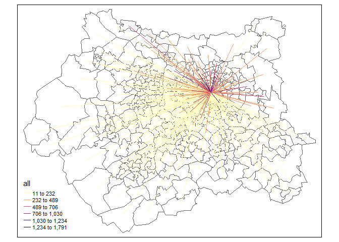
Each row should represent the number of commuters that, every day, go from one MSOA to the same or another MSOA. The data come from 2011 census. For example, in the following map I represent the OD line that "arrive" at "E02006875", which is the code for the MSOA at Leeds city center. Clearly, most of the commuters live nearby their workplace.
tm_shape(west_yorkshire_msoa) +
  tm_borders() +
tm_shape(west_yorkshire_od[west_yorkshire_od$geo_code2 == "E02006875", ]) +
  tm_lines(
    col = "all",
    style = "headtails",
    palette = "-magma",
    style.args = list(thr = 0.5),
    lwd = 1.33
  )
Now I download car crashes data for England
england_crashes_2019 <- get_stats19(2019, output_format = "sf", silent = TRUE)
and filter the events located in the west-yorkshire region. The polygonal boundary for the west-yorkshire region is created by st-unioning the MSOA zones (after rouding all coordinates to the nearest 10s of meter).
st_precision(west_yorkshire_msoa) <- units::set_units(10, "m")
idx <- st_contains(st_union(west_yorkshire_msoa), england_crashes_2019)
west_yorkshire_crashes_2019 <- england_crashes_2019[unlist(idx), ]
I can now count the occurrences in each MSOA
west_yorkshire_msoa$number_of_car_crashes_2019 <- lengths(
  st_contains(west_yorkshire_msoa, west_yorkshire_crashes_2019)
)
and plot the result. The first map represents the location of all car crashes that occurred in the West-Yorkshire during 2019, while the second map is a choropleth map of car crashes counts in each MSOA zone.
p1 <- tm_shape(west_yorkshire_msoa) +
  tm_borders() +
tm_shape(west_yorkshire_crashes_2019) +
  tm_dots(size = 0.005)
p2 <- tm_shape(west_yorkshire_msoa) +
  tm_polygons(
    col = "number_of_car_crashes_2019",
    style = "headtails",
    title = ""
  )
tmap_arrange(p1, p2)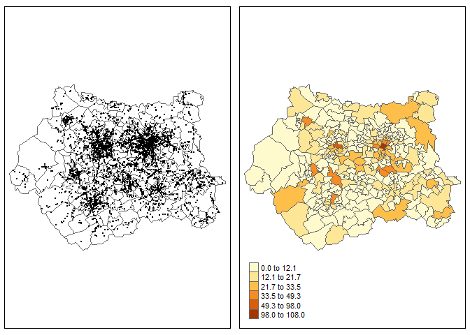
I don't live in Yorkshire but I think that the second map clearly highlights the cities of Leeds, Bradford and Wakefield. The same procedure can be repeated for 2011-2018, creating a simple animation. First I need to download and filter car crashes data for 2011-2019. Warning: the following command may take some time to run
england_crashes_2011_2019 <- get_stats19(2011:2019, output_format = "sf")
idx <- st_contains(st_union(west_yorkshire_msoa), england_crashes_2011_2019)
west_yorkshire_crashes_2011_2019 <- england_crashes_2011_2019[unlist(idx), ]
Then, I need to estimate the number of car crashes per MSOA per year:
west_yorkshire_msoa_spacetime <- do.call("rbind", lapply(
  X = 2011:2019, # the chosen years
  FUN = function(year) {
    id_year <- format(west_yorkshire_crashes_2011_2019$date, "%Y") == as.character(year)
    subset_crashes <- west_yorkshire_crashes_2011_2019[id_year, ]
    st_sf(
      data.frame(
        number_car_crashes = lengths(st_contains(west_yorkshire_msoa, subset_crashes)),
        year = year
      ),
      geometry = st_geometry(west_yorkshire_msoa)
    )
  }
))
And create the animation
tmap_animation(
  tm_shape(west_yorkshire_msoa_spacetime) +
    tm_polygons(col = "number_car_crashes", style = "headtails") +
    tm_facets(along = "year"),
  filename = "tests_tmap.gif",
  delay = 100
)
The car crashes focus more or less always in the same areas (for obvious reasons) and they seem to be more and more focused around the big cities.
Now I want to estimate a traffic measure for each MSOA zone (to be used as an offset in a car crashes model, offtopic here). The problem with raw OD data is that they ignore the fact that people may travel to their workplace through several MSOAs (@Robinlovelace please correct me here). So I estimate a traffic measure using the following approximation. First I build a neighbours list starting from the MSOA regions:
west_yorkshire_queen_nb <- poly2nb(west_yorkshire_msoa, snap = 10)
I think this is more or less equivalent to queen_nb_west_yorkshire <- st_relate(msoa_west_yorkshire, pattern = "F***T****") since we set st_precision(msoa_west_yorkshire) <- units::set_units(10, "m"). I'm not sure how to visualise nb objects with tmap (but I think it could be a nice extension, if absent), so I will use base R + spdep for the moment:
par(mar = rep(0, 4))
plot(st_geometry(west_yorkshire_msoa))
plot(west_yorkshire_queen_nb, st_centroid(st_geometry(west_yorkshire_msoa)), add = TRUE)
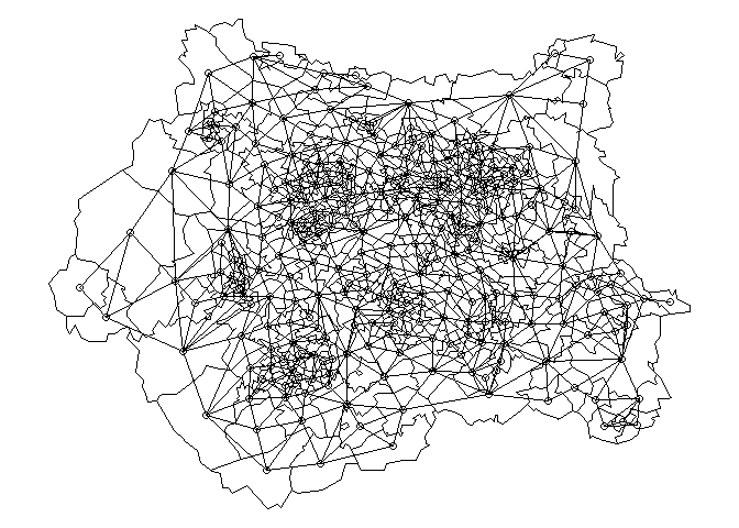
The lines connect the centroid of each MSOA with the centroids of all neighbouring MSOA. This structure is useful since it uniquely determines the adjacency matrix of a graph that can be used to estimate the (approximate) shortest path between two MSOA (i.e. the Origin and the Destination).
west_yorkshire_graph <- graph_from_adjacency_matrix(nb2mat(west_yorkshire_queen_nb, style = "B"))
west_yorkshire_graph
#> IGRAPH b1a7661 D--- 299 1716 --
#> + edges from b1a7661:
#>  [1]  1->  2  1->  3  1->  4  1->  5  1->  6  1-> 10  2->  1  3->  1  3->  5
#> [10]  3->150  3->151  4->  1  4->  6  4->  7  4-> 14  5->  1  5->  3  5->  6
#> [19]  5-> 10  5->151  5->155  6->  1  6->  4  6->  5  6->  7  6->  8  6-> 10
#> [28]  6-> 15  7->  4  7->  6  7->  8  7->  9  7-> 14  8->  6  8->  7  8->  9
#> [37]  8-> 11  8-> 15  8-> 31  9->  7  9->  8  9-> 11  9-> 12  9-> 14 10->  1
#> [46] 10->  5 10->  6 10-> 13 10-> 15 10-> 18 10->155 11->  8 11->  9 11-> 12
#> [55] 11-> 14 11-> 23 11-> 31 12->  9 12-> 11 12-> 14 13-> 10 13-> 16 13-> 17
#> [64] 13-> 18 13->155 14->  4 14->  7 14->  9 14-> 11 14-> 12 14-> 23 15->  6
#> [73] 15->  8 15-> 10 15-> 18 15-> 22 15-> 31 16-> 13 16-> 17 16-> 18 16-> 20
#> + ... omitted several edges
That graph has 299 vertices (the number of MSOA in West Yorkshire) and 1716 edges (the lines visualised in the previous plot). Now I'm going to "decorate" that graph by assigning to each edge a weight that is equal to the geographical distance between the centroids that define the edge. First I need the edgelist:
west_yorkshire_edgelist <- as_edgelist(west_yorkshire_graph)
and then I can estimate the distances
E(west_yorkshire_graph)$weight <- units::drop_units(st_distance(
  x = st_centroid(st_geometry(west_yorkshire_msoa))[west_yorkshire_edgelist[, 1]],
  y = st_centroid(st_geometry(west_yorkshire_msoa))[west_yorkshire_edgelist[, 2]],
  by_element = TRUE
))
I can also assign a name to each vertex equal to the corresponding MSOA code:
V(west_yorkshire_graph)$name <- west_yorkshire_msoa[["geo_code"]]
This is the result, with an analogous interpretation as before
west_yorkshire_graph
#> IGRAPH b1a7661 DNW- 299 1716 --
#> + attr: name (v/c), weight (e/n)
#> + edges from b1a7661 (vertex names):
#>  [1] E02002183->E02002184 E02002183->E02002185 E02002183->E02002186
#>  [4] E02002183->E02002187 E02002183->E02002188 E02002183->E02002192
#>  [7] E02002184->E02002183 E02002185->E02002183 E02002185->E02002187
#> [10] E02002185->E02002332 E02002185->E02002333 E02002186->E02002183
#> [13] E02002186->E02002188 E02002186->E02002189 E02002186->E02002196
#> [16] E02002187->E02002183 E02002187->E02002185 E02002187->E02002188
#> [19] E02002187->E02002192 E02002187->E02002333 E02002187->E02002337
#> [22] E02002188->E02002183 E02002188->E02002186 E02002188->E02002187
#> + ... omitted several edges
Now I'm going to loop over all OD lines, calculate the shortest path between the Origin and Destination MSOA, and assign to each MSOA in the shortest path a traffic measure that is proportional to the number of people that commute using that OD line. I know that it sounds a little confusing but I can write it better if you like the idea:
west_yorkshire_msoa$traffic <- 0 # initialize the traffic column

pb <- txtProgressBar(min = 1, max = nrow(west_yorkshire_od), style = 3)
for (i in seq_len(nrow(west_yorkshire_od))) {
  origin <- west_yorkshire_od[["geo_code1"]][i]
  destination <- west_yorkshire_od[["geo_code2"]][i]

  if (origin == destination) { # this should be an "intrazonal"
    idx <- which(west_yorkshire_msoa$geo_code == origin)
    west_yorkshire_msoa$traffic[idx] <- west_yorkshire_msoa$traffic[idx] + west_yorkshire_od[["all"]][i]
    # west_yorkshire_msoa$traffic[idx] is the previous value while
    # west_yorkshire_od[["all"]][i] is the "new" traffic value
    next()
  }

  # Estimate shortest path
  idx_geo_code <- as_ids(shortest_paths(west_yorkshire_graph, from = origin, to = destination)$vpath[[1]])
  idx <- which(west_yorkshire_msoa$geo_code %in% idx_geo_code)
  west_yorkshire_msoa$traffic[idx] <- west_yorkshire_msoa$traffic[idx] + (west_yorkshire_od[["all"]][i] / length(idx))
  # west_yorkshire_msoa$traffic[idx] are the previous values while
  # west_yorkshire_od[["all"]][i] is the new traffic count (divided by the
  # number of MSOAs in the shortest path)

  setTxtProgressBar(pb, i)
}
For example, if i = 53778, then
west_yorkshire_od[53778, 1:3]
#> Simple feature collection with 1 feature and 3 fields
#> geometry type:  LINESTRING
#> dimension:      XY
#> bbox:           xmin: 415279.3 ymin: 418009.9 xmax: 430001.7 ymax: 433379.7
#> projected CRS:  OSGB 1936 / British National Grid
#>       geo_code1 geo_code2 all                       geometry
#> 53778 E02006875 E02002299  18 LINESTRING (430001.7 433379...
i.e. the number of daily commuters is equal to 18, while the shortest path between E02006875 and E02002299 is given by
shortest_path_example <- shortest_paths(west_yorkshire_graph, "E02006875", "E02002299", output = "both")
shortest_path_example
#> $vpath
#> $vpath[[1]]
#> + 12/299 vertices, named, from b1a7661:
#>  [1] E02006875 E02002411 E02002419 E02002422 E02002433 E02002435 E02002276
#>  [8] E02002281 E02002285 E02002302 E02002307 E02002299
#>
#>
#> $epath
#> $epath[[1]]
#> + 11/1716 edges from b1a7661 (vertex names):
#>  [1] E02006875->E02002411 E02002411->E02002419 E02002419->E02002422
#>  [4] E02002422->E02002433 E02002433->E02002435 E02002435->E02002276
#>  [7] E02002276->E02002281 E02002281->E02002285 E02002285->E02002302
#> [10] E02002302->E02002307 E02002307->E02002299
#>
#>
#> $predecessors
#> NULL
#>
#> $inbound_edges
#> NULL
It would be nice to represent the "shortest path" like the previous map (and check the results) but I'm not sure how to do that right now.
Now, we can compare the traffic estimates with the car crashes counts:
p1 <- tm_shape(west_yorkshire_msoa) +
  tm_polygons(
    col = "number_of_car_crashes_2019",
    style = "headtails",
    title = ""
  )
p2 <- tm_shape(west_yorkshire_msoa) +
  tm_polygons(
    col = "traffic",
    style = "headtails",
    title = ""
  )
tmap_arrange(p1, p2)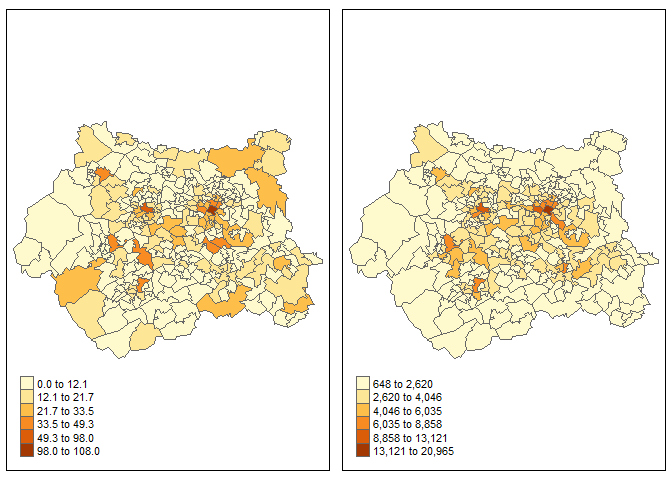
The scales are quite different (obviously), but they highlight the same areas (which is not incredible, but still...)
I think that the examples presented here are nice since they are related to a "real-world application" with open data (with some licence limitation maybe, I don't know). I think that the visualisation component should be stressed much more (and the maps related to neighborhood matrices should be implemented with tmap). This example is probably too difficult for a book not related to road safety or models for car crashes, but if you like it I think we can organize something!
Created on 2020-10-10 by the reprex package (v0.3.0)
Session info
devtools::session_info()
#> - Session info ---------------------------------------------------------------
#>  setting  value
#>  version  R version 3.6.3 (2020-02-29)
#>  os       Windows 10 x64
#>  system   x86_64, mingw32
#>  ui       RTerm
#>  language (EN)
#>  collate  Italian_Italy.1252
#>  ctype    Italian_Italy.1252
#>  tz       Europe/Berlin
#>  date     2020-10-10
#>
#> - Packages -------------------------------------------------------------------
#>  package      * version    date       lib source
#>  abind          1.4-5      2016-07-21 [1] CRAN (R 3.6.0)
#>  assertthat     0.2.1      2019-03-21 [1] CRAN (R 3.6.0)
#>  backports      1.1.10     2020-09-15 [1] CRAN (R 3.6.3)
#>  base64enc      0.1-3      2015-07-28 [1] CRAN (R 3.6.0)
#>  boot           1.3-25     2020-04-26 [1] CRAN (R 3.6.3)
#>  callr          3.4.4      2020-09-07 [1] CRAN (R 3.6.3)
#>  class          7.3-17     2020-04-26 [1] CRAN (R 3.6.3)
#>  classInt       0.4-3      2020-04-07 [1] CRAN (R 3.6.3)
#>  cli            2.0.2      2020-02-28 [1] CRAN (R 3.6.3)
#>  coda           0.19-3     2019-07-05 [1] CRAN (R 3.6.1)
#>  codetools      0.2-16     2018-12-24 [2] CRAN (R 3.6.3)
#>  crayon         1.3.4      2017-09-16 [1] CRAN (R 3.6.0)
#>  crosstalk      1.1.0.1    2020-03-13 [1] CRAN (R 3.6.3)
#>  curl           4.3        2019-12-02 [1] CRAN (R 3.6.1)
#>  DBI            1.1.0      2019-12-15 [1] CRAN (R 3.6.3)
#>  deldir         0.1-29     2020-09-13 [1] CRAN (R 3.6.3)
#>  desc           1.2.0      2018-05-01 [1] CRAN (R 3.6.0)
#>  devtools       2.3.2      2020-09-18 [1] CRAN (R 3.6.3)
#>  dichromat      2.0-0      2013-01-24 [1] CRAN (R 3.6.0)
#>  digest         0.6.25     2020-02-23 [1] CRAN (R 3.6.3)
#>  dplyr          1.0.2      2020-08-18 [1] CRAN (R 3.6.3)
#>  e1071          1.7-3      2019-11-26 [1] CRAN (R 3.6.1)
#>  ellipsis       0.3.1      2020-05-15 [1] CRAN (R 3.6.3)
#>  evaluate       0.14       2019-05-28 [1] CRAN (R 3.6.0)
#>  expm           0.999-5    2020-07-20 [1] CRAN (R 3.6.3)
#>  fansi          0.4.1      2020-01-08 [1] CRAN (R 3.6.2)
#>  fs             1.5.0      2020-07-31 [1] CRAN (R 3.6.3)
#>  gdata          2.18.0     2017-06-06 [1] CRAN (R 3.6.0)
#>  generics       0.0.2      2018-11-29 [1] CRAN (R 3.6.0)
#>  gifski         0.8.6      2018-09-28 [1] CRAN (R 3.6.0)
#>  glue           1.4.2      2020-08-27 [1] CRAN (R 3.6.3)
#>  gmodels        2.18.1     2018-06-25 [1] CRAN (R 3.6.1)
#>  gtools         3.8.2      2020-03-31 [1] CRAN (R 3.6.3)
#>  highr          0.8        2019-03-20 [1] CRAN (R 3.6.0)
#>  hms            0.5.3      2020-01-08 [1] CRAN (R 3.6.2)
#>  htmltools      0.5.0      2020-06-16 [1] CRAN (R 3.6.3)
#>  htmlwidgets    1.5.1      2019-10-08 [1] CRAN (R 3.6.1)
#>  httr           1.4.2      2020-07-20 [1] CRAN (R 3.6.3)
#>  igraph       * 1.2.5      2020-03-19 [1] CRAN (R 3.6.3)
#>  KernSmooth     2.23-17    2020-04-26 [1] CRAN (R 3.6.3)
#>  knitr          1.30       2020-09-22 [1] CRAN (R 3.6.3)
#>  lattice        0.20-41    2020-04-02 [1] CRAN (R 3.6.3)
#>  leafem         0.1.3      2020-07-26 [1] CRAN (R 3.6.3)
#>  leaflet        2.0.3      2019-11-16 [1] CRAN (R 3.6.3)
#>  leafsync       0.1.0      2019-03-05 [1] CRAN (R 3.6.1)
#>  LearnBayes     2.15.1     2018-03-18 [1] CRAN (R 3.6.0)
#>  lifecycle      0.2.0      2020-03-06 [1] CRAN (R 3.6.2)
#>  lwgeom         0.2-5      2020-06-12 [1] CRAN (R 3.6.3)
#>  magrittr       1.5        2014-11-22 [1] CRAN (R 3.6.3)
#>  MASS           7.3-53     2020-09-09 [1] CRAN (R 3.6.3)
#>  Matrix         1.2-18     2019-11-27 [2] CRAN (R 3.6.3)
#>  memoise        1.1.0      2017-04-21 [1] CRAN (R 3.6.0)
#>  mime           0.9        2020-02-04 [1] CRAN (R 3.6.2)
#>  nlme           3.1-149    2020-08-23 [1] CRAN (R 3.6.3)
#>  od           * 0.0.1      2020-09-09 [1] CRAN (R 3.6.3)
#>  pct          * 0.5.0      2020-08-27 [1] CRAN (R 3.6.3)
#>  pillar         1.4.6      2020-07-10 [1] CRAN (R 3.6.3)
#>  pkgbuild       1.1.0      2020-07-13 [1] CRAN (R 3.6.3)
#>  pkgconfig      2.0.3      2019-09-22 [1] CRAN (R 3.6.1)
#>  pkgload        1.1.0      2020-05-29 [1] CRAN (R 3.6.3)
#>  png            0.1-7      2013-12-03 [1] CRAN (R 3.6.0)
#>  prettyunits    1.1.1      2020-01-24 [1] CRAN (R 3.6.2)
#>  processx       3.4.4      2020-09-03 [1] CRAN (R 3.6.3)
#>  ps             1.3.4      2020-08-11 [1] CRAN (R 3.6.3)
#>  purrr          0.3.4      2020-04-17 [1] CRAN (R 3.6.3)
#>  R6             2.4.1      2019-11-12 [1] CRAN (R 3.6.1)
#>  raster         3.3-13     2020-07-17 [1] CRAN (R 3.6.3)
#>  RColorBrewer   1.1-2      2014-12-07 [1] CRAN (R 3.6.0)
#>  Rcpp           1.0.5      2020-07-06 [1] CRAN (R 3.6.3)
#>  readr          1.3.1      2018-12-21 [1] CRAN (R 3.6.0)
#>  remotes        2.2.0      2020-07-21 [1] CRAN (R 3.6.3)
#>  rlang          0.4.7      2020-07-09 [1] CRAN (R 3.6.3)
#>  rmarkdown      2.3        2020-06-18 [1] CRAN (R 3.6.3)
#>  rprojroot      1.3-2      2018-01-03 [1] CRAN (R 3.6.0)
#>  sessioninfo    1.1.1      2018-11-05 [1] CRAN (R 3.6.0)
#>  sf           * 0.9-6      2020-09-13 [1] CRAN (R 3.6.3)
#>  sfheaders      0.2.2      2020-05-13 [1] CRAN (R 3.6.3)
#>  sp           * 1.4-2      2020-05-20 [1] CRAN (R 3.6.3)
#>  spData       * 0.3.8      2020-07-03 [1] CRAN (R 3.6.3)
#>  spDataLarge    0.3.1      2019-06-30 [1] Github (Nowosad/spDataLarge@012fe53)
#>  spdep        * 1.1-5      2020-06-29 [1] CRAN (R 3.6.3)
#>  stars          0.4-4      2020-08-19 [1] Github (r-spatial/stars@b7b54c8)
#>  stats19      * 1.3.0      2020-09-30 [1] local
#>  stringi        1.4.6      2020-02-17 [1] CRAN (R 3.6.2)
#>  stringr        1.4.0      2019-02-10 [1] CRAN (R 3.6.0)
#>  testthat       2.3.2      2020-03-02 [1] CRAN (R 3.6.3)
#>  tibble         3.0.3.9000 2020-07-12 [1] Github (tidyverse/tibble@a57ad4a)
#>  tidyselect     1.1.0      2020-05-11 [1] CRAN (R 3.6.3)
#>  tmap         * 3.2        2020-09-15 [1] CRAN (R 3.6.3)
#>  tmaptools      3.1        2020-07-12 [1] Github (mtennekes/tmaptools@947f3bd)
#>  units          0.6-7      2020-06-13 [1] CRAN (R 3.6.3)
#>  usethis        1.6.3      2020-09-17 [1] CRAN (R 3.6.3)
#>  vctrs          0.3.4      2020-08-29 [1] CRAN (R 3.6.3)
#>  viridisLite    0.3.0      2018-02-01 [1] CRAN (R 3.6.0)
#>  withr          2.3.0      2020-09-22 [1] CRAN (R 3.6.3)
#>  xfun           0.17       2020-09-09 [1] CRAN (R 3.6.3)
#>  XML            3.99-0.3   2020-01-20 [1] CRAN (R 3.6.2)
#>  xml2           1.3.2      2020-04-23 [1] CRAN (R 3.6.3)
#>  yaml           2.2.1      2020-02-01 [1] CRAN (R 3.6.2)
#>
#> [1] C:/Users/Utente/Documents/R/win-library/3.6
#> [2] C:/Program Files/R/R-3.6.3/library
Hi! The following reprex should present the datasets.
First, I download MSOA data for the West-Yorkshire region (polygonal data)
The MSOA areas are defined here. Then, I download OD data for the West-Yorkshire region
and transform them, adding a LINESTRING between the centroids of each pair of MSOAs
This is the result
Each row should represent the number of commuters that, every day, go from one MSOA to the same or another MSOA. The data come from 2011 census. For example, in the following map I represent the OD line that "arrive" at "E02006875", which is the code for the MSOA at Leeds city center. Clearly, most of the commuters live nearby their workplace.
Now I download car crashes data for England
and filter the events located in the west-yorkshire region. The polygonal boundary for the west-yorkshire region is created by st-unioning the MSOA zones (after rouding all coordinates to the nearest 10s of meter).
I can now count the occurrences in each MSOA
and plot the result. The first map represents the location of all car crashes that occurred in the West-Yorkshire during 2019, while the second map is a choropleth map of car crashes counts in each MSOA zone.
I don't live in Yorkshire but I think that the second map clearly highlights the cities of Leeds, Bradford and Wakefield. The same procedure can be repeated for 2011-2018, creating a simple animation. First I need to download and filter car crashes data for 2011-2019. Warning: the following command may take some time to run
Then, I need to estimate the number of car crashes per MSOA per year:
And create the animation
The car crashes focus more or less always in the same areas (for obvious reasons) and they seem to be more and more focused around the big cities.
Now I want to estimate a traffic measure for each MSOA zone (to be used as an offset in a car crashes model, offtopic here). The problem with raw OD data is that they ignore the fact that people may travel to their workplace through several MSOAs (@Robinlovelace please correct me here). So I estimate a traffic measure using the following approximation. First I build a neighbours list starting from the MSOA regions:
I think this is more or less equivalent to
queen_nb_west_yorkshire <- st_relate(msoa_west_yorkshire, pattern = "F***T****")since we setst_precision(msoa_west_yorkshire) <- units::set_units(10, "m"). I'm not sure how to visualisenbobjects withtmap(but I think it could be a nice extension, if absent), so I will use base R +spdepfor the moment:The lines connect the centroid of each MSOA with the centroids of all neighbouring MSOA. This structure is useful since it uniquely determines the adjacency matrix of a graph that can be used to estimate the (approximate) shortest path between two MSOA (i.e. the Origin and the Destination).
That graph has 299 vertices (the number of MSOA in West Yorkshire) and 1716 edges (the lines visualised in the previous plot). Now I'm going to "decorate" that graph by assigning to each edge a weight that is equal to the geographical distance between the centroids that define the edge. First I need the edgelist:
and then I can estimate the distances
I can also assign a name to each vertex equal to the corresponding MSOA code:
This is the result, with an analogous interpretation as before
Now I'm going to loop over all OD lines, calculate the shortest path between the Origin and Destination MSOA, and assign to each MSOA in the shortest path a traffic measure that is proportional to the number of people that commute using that OD line. I know that it sounds a little confusing but I can write it better if you like the idea:
For example, if
i = 53778, theni.e. the number of daily commuters is equal to 18, while the shortest path between E02006875 and E02002299 is given by
It would be nice to represent the "shortest path" like the previous map (and check the results) but I'm not sure how to do that right now.
Now, we can compare the traffic estimates with the car crashes counts:
The scales are quite different (obviously), but they highlight the same areas (which is not incredible, but still...)
I think that the examples presented here are nice since they are related to a "real-world application" with open data (with some licence limitation maybe, I don't know). I think that the visualisation component should be stressed much more (and the maps related to neighborhood matrices should be implemented with
tmap). This example is probably too difficult for a book not related to road safety or models for car crashes, but if you like it I think we can organize something!Created on 2020-10-10 by the reprex package (v0.3.0)
Session info