018‐ scATAC‐Seq
Single cell ATAC sequencing with scRNA-Seq (scATAC-Seq)
library("iCellR")
my.data <- load10x("filtered_gene_bc_matrices/")

# see the row names
row.names(my.data)

# get peak names
ATAC <- grep("^chr",row.names(my.data),value=T)

# get scATAC data
MyATAC <- subset(my.data, row.names(my.data) %in% ATAC)
head(MyATAC)[1:3]
#                   AAACAGCCAAGTGAAC.1 AAACAGCCACTGACCG.1 AAACAGCCATGATTGT.1
#chr1.181218.181695                  0                  0                  1
#chr1.191296.191699                  0                  0                  0
#chr1.629770.630129                  0                  0                  0
#chr1.633806.634251                  0                  0                  0
#chr1.778422.779040                  0                  0                  0
#chr1.827306.827702                  0                  0                  0

dim(MyATAC)
# [1] 21923  6326

# get RNA data
MyRNAs <- subset(my.data, !row.names(my.data) %in% ATAC)
head(MyRNAs)[1:3]
#            AAACAGCCAAGTGAAC.1 AAACAGCCACTGACCG.1 AAACAGCCATGATTGT.1
#MIR1302.2HG                  0                  0                  0
#FAM138A                      0                  0                  0
#OR4F5                        0                  0                  0
#AL627309.1                   0                  0                  0
#AL627309.3                   0                  0                  0
#AL627309.2                   0                  0                  0

dim(MyRNAs)
#[1] 36633  6326

# make iCellR object
my.obj <- make.obj(MyRNAs)

# add ATAC-Seq data
my.obj@atac.raw <- MyATAC
my.obj@atac.main <- MyATAC

# check your object
my.obj


###################################
,--. ,-----.       ,--.,--.,------.
`--''  .--./ ,---. |  ||  ||  .--. '
,--.|  |    | .-. :|  ||  ||  '--'.'
|  |'  '--'\   --. |  ||  ||  |
`--' `-----' `----'`--'`--'`--' '--'
###################################
An object of class iCellR version: 1.6.2
Raw/original data dimentions (rows,columns): 24127,6326
Data conditions: no conditions/single sample
Row names: MIR1302.2HG,TTLL10.AS1,MRPL20.AS1 ...
Columns names: AAACAGCCAAGTGAAC.1,AAACAGCCACTGACCG.1,AAACAGCCATGATTGT.1 ...
###################################
   QC stats performed:FALSE, PCA performed:FALSE
   Clustering performed:FALSE, Number of clusters:0
   tSNE performed:FALSE, UMAP performed:FALSE, DiffMap performed:FALSE
   Main data dimensions (rows,columns): 0,0
   Normalization factors:,...
   Imputed data dimensions (rows,columns):0,0
############## scVDJ-seq ###########
VDJ data dimentions (rows,columns):0,0
############## CITE-seq ############
   ADT raw data  dimensions (rows,columns):0,0
   ADT main data  dimensions (rows,columns):0,0
   ADT columns names:...
   ADT row names:...
############## scATAC-seq ############
   ATAC raw data  dimensions (rows,columns):21923,6326
   ATAC main data  dimensions (rows,columns):21923,6326
   ATAC columns names:AAACAGCCAAGTGAAC.1...
   ATAC row names:chr1.181218.181695...
############## Spatial ###########
Spatial data dimentions (rows,columns):0,0
########### iCellR object ##########
From here do the regular scRNA-seq as expleind above. See example below
# QC
my.obj <- qc.stats(my.obj,
   s.phase.genes = s.phase,
   g2m.phase.genes = g2m.phase)

# plot as mentioned above

# filter
my.obj <- cell.filter(my.obj,
   min.mito = 0,
   max.mito = 0.07 ,
   min.genes = 500,
   max.genes = 4000,
   min.umis = 0,
   max.umis = Inf)

# normalize RNA
my.obj <- norm.data(my.obj, norm.method = "ranked.glsf", top.rank = 500)

# normalize ADT
my.obj <- norm.adt(my.obj)

# gene stats
my.obj <- gene.stats(my.obj, which.data = "main.data")

# find genes for PCA
my.obj <- make.gene.model(my.obj, my.out.put = "data",
   dispersion.limit = 1.5,
   base.mean.rank = 500,
   no.mito.model = T,
   mark.mito = T,
   interactive = F,
   no.cell.cycle = T,
   out.name = "gene.model")

# run PCA and the rest is as above

my.obj <- run.pca(my.obj, method = "gene.model", gene.list = my.obj@gene.model,data.type = "main")

# tSNE
my.obj <- run.pc.tsne(my.obj, dims = 1:10)

# UMAP
my.obj <- run.umap(my.obj, dims = 1:10)

# KNetL
my.obj <- run.knetl(my.obj, dims = 1:20, zoom = 200, dim.redux = "umap")

# clustering based on KNetL

my.obj <- iclust(my.obj, sensitivity = 200, data.type = "knetl")

# clustering based on PCA

# my.obj <- iclust(my.obj, sensitivity = 100, data.type = "pca", dims=1:10)

# check clusters and adjust if needed (optinal)
# cluster.plot(my.obj,plot.type = "knetl",interactive = F,cell.size = 0.5,cell.transparency = 1, anno.clust=T)
# my.obj <- change.clust(my.obj, change.clust = 3, to.clust = 4)
# my.obj <- change.clust(my.obj, change.clust = 3, to.clust = 10)

# order clusters
my.obj <- clust.ord(my.obj,top.rank = 500, how.to.order = "distance")


# plot
A= cluster.plot(my.obj,plot.type = "pca",interactive = F,cell.size = 0.5,cell.transparency = 1, anno.clust=T)
B= cluster.plot(my.obj,plot.type = "umap",interactive = F,cell.size = 0.5,cell.transparency = 1, anno.clust=T)
C= cluster.plot(my.obj,plot.type = "tsne",interactive = F,cell.size = 0.5,cell.transparency = 1, anno.clust=T)
D= cluster.plot(my.obj,plot.type = "knetl",interactive = F,cell.size = 0.5,cell.transparency = 1, anno.clust=T)

library(gridExtra)
png('AllClusts.png', width = 12, height = 10, units = 'in', res = 300)
grid.arrange(A,B,C,D)
dev.off()

# save object
save(my.obj, file = "my.obj.Robj")

# find markers
marker.genes <- findMarkers(my.obj,
data.type = "main",
fold.change = 2,
padjval = 0.1,
uniq = F,
positive = T)

marker.genes1 <- cbind(row = rownames(marker.genes), marker.genes)
write.table((marker.genes1),file="marker.genes.tsv", sep="\t", row.names =F)

MyGenes <- top.markers(marker.genes, topde = 10, min.base.mean = 0.2, filt.ambig = F)
MyGenes <- unique(MyGenes)

png('heatmap_gg_genes.png', width = 10, height = 10, units = 'in', res = 300)
heatmap.gg.plot(my.obj, gene = MyGenes, interactive = F, cluster.by = "clusters",cell.sort = F, conds.to.plot = NULL)
dev.off()
Work on scATAC data (normalize and find marker peaks for each cluster)
# normalize ACAT
my.obj <- norm.data(my.obj, norm.method = "ranked.glsf", top.rank = 500, ATAC.data = TRUE, ATAC.filter = TRUE)

marker.peaks <- findMarkers(my.obj,
 data.type = "atac",
 fold.change = 2,
 padjval = 0.1,
 uniq = F,
 positive = T)

marker.peaks1 <- cbind(row = rownames(marker.peaks), marker.peaks)
write.table((marker.peaks1),file="marker.peaks.tsv", sep="\t", row.names =F)

head(marker.peaks1)
#                                             row   baseMean     baseSD
#chr17.64986035.64986113   chr17.64986035.64986113 0.01217359 0.18257818
#chr1.26542287.26542678     chr1.26542287.26542678 0.05828764 0.80077656
#chr4.8199063.8199275         chr4.8199063.8199275 0.04280424 0.56205649
#chr20.50274929.50275237   chr20.50274929.50275237 0.04684509 0.63361490
#chr2.218382038.218382236 chr2.218382038.218382236 0.03122394 0.31153105
#chr11.1760469.1760814       chr11.1760469.1760814 0.07050175 0.63322284
#                         AvExpInCluster AvExpInOtherClusters foldChange
#chr17.64986035.64986113      0.07868394          0.002346603  33.530999
#chr1.26542287.26542678       0.33849093          0.016887273  20.044144
#chr4.8199063.8199275         0.24803497          0.012481148  19.872769
#chr20.50274929.50275237      0.27007513          0.013862584  19.482308
#chr2.218382038.218382236     0.17736269          0.009631770  18.414340
#chr11.1760469.1760814        0.39043782          0.023230813  16.806894
#                         log2FoldChange         pval         padj clusters
#chr17.64986035.64986113        5.067424 1.187697e-05 2.875415e-02        1
#chr1.26542287.26542678         4.325109 3.653916e-05 8.539202e-02        1
#chr4.8199063.8199275           4.312721 6.059691e-06 1.489472e-02        1
#chr20.50274929.50275237        4.284093 2.871301e-05 6.779143e-02        1
#chr2.218382038.218382236       4.202758 6.359572e-10 1.677019e-06        1
#chr11.1760469.1760814          4.070981 6.813447e-11 1.800794e-07        1
#                                             gene    cluster_1   cluster_2
#chr17.64986035.64986113   chr17.64986035.64986113 0.0786839378 0.000000000
#chr1.26542287.26542678     chr1.26542287.26542678 0.3384909326 0.008895062
#chr4.8199063.8199275         chr4.8199063.8199275 0.2480349741 0.038672840
#chr20.50274929.50275237   chr20.50274929.50275237 0.2700751295 0.028703704
#chr2.218382038.218382236 chr2.218382038.218382236 0.1773626943 0.000000000
#chr11.1760469.1760814       chr11.1760469.1760814 0.3904378238 0.004537037
#                           cluster_3    cluster_4    cluster_5    cluster_6
#chr17.64986035.64986113  0.000000000 0.0000000000 0.0006934750 0.0010038760
#chr1.26542287.26542678   0.031485714 0.0029244992 0.0052261002 0.0041264535
#chr4.8199063.8199275     0.000000000 0.0007226502 0.0027450683 0.0113212209
#chr20.50274929.50275237  0.027092857 0.0121741140 0.0041820941 0.0051516473
#chr2.218382038.218382236 0.004292857 0.0042095532 0.0006722307 0.0038561047
#chr11.1760469.1760814    0.071678571 0.0177288136 0.0141820941 0.0061099806
#                           cluster_7   cluster_8
#chr17.64986035.64986113  0.003099029 0.009080357
#chr1.26542287.26542678   0.047110680 0.044484375
#chr4.8199063.8199275     0.014819417 0.028651786
#chr20.50274929.50275237  0.025499029 0.028765625
#chr2.218382038.218382236 0.011988350 0.035508929
#chr11.1760469.1760814    0.042093204 0.050708705

MyGenes <- top.markers(marker.peaks, topde = 10, min.base.mean = 0.2, filt.ambig = F)
MyGenes <- unique(MyGenes)

png('heatmap_gg_peaks.png', width = 10, height = 10, units = 'in', res = 300)
heatmap.gg.plot(my.obj, gene = MyGenes, interactive = F, cluster.by = "clusters",cell.sort = F, conds.to.plot = NULL, data.type = "atac")
dev.off()

my.obj <- run.impute(my.obj,data.type = "knetl", nn = 10, ATAC.data = FALSE)


png('heatmap_gg_peaks.png', width = 10, height = 10, units = 'in', res = 300)
heatmap.gg.plot(my.obj, gene = MyGenes, interactive = F, cluster.by = "clusters",cell.sort = F, conds.to.plot = NULL, data.type = "atac.imputed")
dev.off()

## you can also find avarage peak intensity per cluster

my.obj <- clust.avg.exp(my.obj, data.type = "atac")
head(my.obj@clust.avg)

#gene  cluster_1  cluster_2	...
#chr1.100037799.100038931 0.38238731 0.36750000	...
#chr1.100132733.100133298 0.11195725 1.13593827	...
#chr1.100249637.100250160 0.09851425 0.09511728	...
#chr1.100265992.100266479 0.06768394 0.17707407	...
#chr1.10032488.10033387 0.35273705 0.14885802	...
#chr1.100352150.100352921 0.12006088 0.00000000	...

# find out which cluster has the highest number

dat <- as.data.frame(t((my.obj@clust.avg)[,-1]))
dat <- hto.anno(hto.data = dat)

head(dat$assignment.annotatio)
#[1] cluster_1 cluster_2 cluster_4 cluster_2 cluster_3 cluster_4
#8 Levels: cluster_1 cluster_2 cluster_3 cluster_4 cluster_5 ... cluster_8
Peak analysis
# make a bed file per cluster from the marker.peaks file you made up here
make.bed(marker.peaks)

# load packages
library(ChIPseeker)
library(clusterProfiler)

# load genome
require(TxDb.Hsapiens.UCSC.hg38.knownGene)
txdb <- TxDb.Hsapiens.UCSC.hg38.knownGene
Anno="org.Hs.eg.db"

# load bed files
Mylist1 = list.files(pattern=".bed")
Mylist1

Mylist <- as.list(Mylist1)
NAMES <- gsub('_peaks.bed','',Mylist1)
names(Mylist) <- NAMES
files <- Mylist
files

# perform analysis (example)
promoter <- getPromoters(TxDb=txdb, upstream=3000, downstream=3000)
tagMatrixList <- lapply(files, getTagMatrix, windows=promoter)

pdf("Plot_ProfileLineAll.pdf")
plotAvgProf(tagMatrixList, xlim=c(-3000, 3000))
dev.off()

pdf('Plot_ProfileLine.pdf', width = 8, height = 10)
plotAvgProf(tagMatrixList, xlim=c(-3000, 3000), facet="row")
dev.off()

pdf("Plot_heatmaps.pdf", width = 50, height = 6)
tagHeatmap(tagMatrixList, xlim=c(-3000, 3000), color=NULL)
dev.off()

# annotate
peakAnnoList <- lapply(files, annotatePeak, TxDb=txdb,
                       tssRegion=c(-3000, 3000), verbose=FALSE)
# plot annotatin
pdf("Plot_AnnoBar.pdf")
plotAnnoBar(peakAnnoList)
dev.off()

############### peak annotation

peakAnnoList <- lapply(files, annotatePeak, TxDb=txdb,
                       tssRegion=c(-3000, 3000), verbose=FALSE, annoDb=Anno)

capture.output(peakAnnoList, file = "peakAnnoList.txt")

genes = lapply(peakAnnoList, function(i) as.data.frame(i))

lapply(1:length(genes), function(i) write.table(genes[[i]],
                                      file = paste0(names(genes[i]), ".xls"),
                                      row.names = FALSE, sep="\t"))
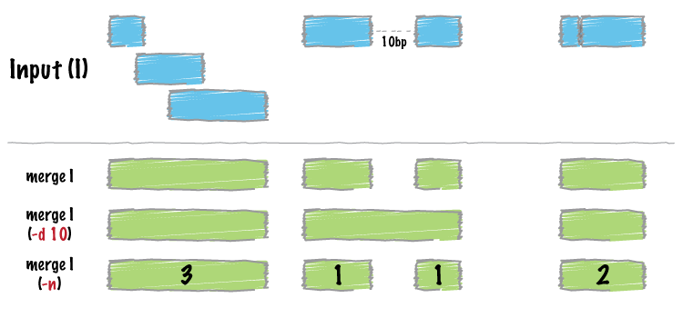
Merging scATAC files with different intervals (as dipicted in bedtools website)
# Let's say you have 2 files that you need to merege

# example file
C <- load10x("count-JJsn_C_cDNA/",gene.name = 2)
M <- load10x("count-JJsn_M_cDNA/",gene.name = 2)

ATAC.C <- grep("^chr",row.names(C),value=T)
ATAC.M <- grep("^chr",row.names(M),value=T)

MyATAC.C <- subset(C, row.names(C) %in% ATAC.C)
MyATAC.M <- subset(M, row.names(M) %in% ATAC.M)

head(MyATAC.C)[1:3]

C <- MyATAC.C
M <- MyATAC.M

dim(C)
#[1] 58678  4211
dim(M)
#[1] 57776  4736

f1 <- row.names(C)
f2 <- row.names(M)

all.peaks <- c(f1,f2)
length(all.peaks)
#[1] 116454

# make a bed file
chr <- as.character(as.matrix(data.frame(do.call('rbind', strsplit(as.character(all.peaks),'.',fixed=TRUE)))[1]))
start <- data.frame(do.call('rbind', strsplit(as.character(all.peaks),'.',fixed=TRUE)))[2]
end <- data.frame(do.call('rbind', strsplit(as.character(all.peaks),'.',fixed=TRUE)))[3]

DAT <- as.data.frame(chr)
DAT$start <- as.numeric(as.matrix(start))
DAT$end <- as.numeric(as.matrix(end))
head(DAT)
#   chr  start    end
#1 chr1 181218 181695
#2 chr1 191296 191699
#3 chr1 629770 630129
#4 chr1 633806 634251
#5 chr1 778422 779040
#6 chr1 827306 827702

# make Genomic Ranges
library("GenomicRanges")

all.gr <- GRanges(seqnames=DAT$chr,ranges=IRanges(start=DAT$start,end=DAT$end))

all.gr
#GRanges object with ?? ranges and 0 metadata columns:
#       seqnames          ranges strand
#          <Rle>       <IRanges>  <Rle>
#   [1]     chr1   181218-181695      *
#   [2]     chr1   191296-191699      *
#   [3]     chr1   629770-630129      *
#   [4]     chr1   633806-634251      *
#   [5]     chr1   778422-779040      *
#   ...      ...             ...    ...
#  [52]     chr1 1303892-1306216      *
#  [53]     chr1 1307242-1309359      *
#  [54]     chr1 1324425-1325236      *
#  [55]     chr1 1348940-1349958      *
#  [56]     chr1 1372031-1372220      *
#  -------
#  seqinfo: 1 sequence from an unspecified genome; no seqlengths

################## sort and merge the peaks

mrg <- reduce(all.gr)

#Before merge
length(all.gr)
#[1] 116454
#after merge
length(mrg)
#[1] 71426

########################## choose file and give name
MyFile <- f1
name="f1_new.bed"
########################## copy paste the code here to make a new bed file
########################## the new bed has the old and new intervals (new intervals to be replaced with old)

chr <- as.character(as.matrix(data.frame(do.call('rbind', strsplit(as.character(MyFile),'.',fixed=TRUE)))[1]))
start <- data.frame(do.call('rbind', strsplit(as.character(MyFile),'.',fixed=TRUE)))[2]
end <- data.frame(do.call('rbind', strsplit(as.character(MyFile),'.',fixed=TRUE)))[3]
# make a bed file
DAT <- as.data.frame(chr)
DAT$start <- as.numeric(as.matrix(start))
DAT$end <- as.numeric(as.matrix(end))
MyFile <- DAT

# make intrval file to replace to new regions
MyFile.gr <- GRanges(seqnames=MyFile$chr,ranges=IRanges(start=MyFile$start,end=MyFile$end))

OverLap <- findOverlaps(MyFile.gr, mrg)

OLD1 <- (OverLap@from)
NEW1 <- (OverLap@to)

OLD = MyFile.gr[OLD1]
NEW = mrg[NEW1]

chr <- as.character(OLD@seqnames)
DAT <- as.data.frame(chr)
DAT$start <- OLD@ranges@start
DAT$end <- (OLD@ranges@start + OLD@ranges@width) - 1

DAT$new.chr<- as.character(NEW@seqnames)
DAT$new.start <- NEW@ranges@start
DAT$new.end <- (NEW@ranges@start + NEW@ranges@width) - 1

head(DAT)
#   chr   start     end new.chr new.start new.end
#1 chr1 3247563 3248453    chr1   3247563 3248453
#2 chr1 3360706 3361554    chr1   3360706 3361554
#3 chr1 3552372 3553230    chr1   3552372 3553230
#4 chr1 3645171 3646034    chr1   3645093 3646034
#5 chr1 3670318 3671081    chr1   3670318 3671090
#6 chr1 3671326 3672230    chr1   3671314 3672230

dim(DAT)
#58678     6
length(MyFile.gr)
#58678

# diff

have = mrg[unique(NEW1)]
dontHave = mrg[-unique(NEW1)]

ADD <- dontHave
L <- length(as.character(ADD@seqnames))
chr <-rep("NA",L)
DAT1 <- as.data.frame(chr)
DAT1$start <- rep("NA",L)
DAT1$end <- rep("NA",L)
DAT1$new.chr<- as.character(ADD@seqnames)
DAT1$new.start <- ADD@ranges@start
DAT1$new.end <- (ADD@ranges@start + ADD@ranges@width) - 1

Final.DAT <- rbind(DAT,DAT1)

##### Write

write.table(Final.DAT,name,row.names=FALSE,sep="\t", quote = FALSE)

### reapeat this process for f2 (M) as well

# The first 3 columns are the original peaks and the last 3 are the ones that need to be replaced with original one. The NA peaks would also get the new peak ids but in the matrix the cells will have 0 for expressions. To do this use the iCellR function replace.peak.id.

MyATAC.C <- replace.peak.id(atac.data=MyATAC.C, bed.file = Final.DAT.C)
MyATAC.M <- replace.peak.id(atac.data=MyATAC.M, bed.file = Final.DAT.M)

# finally aggregate the samples and add to iCellR object

my.atac.data <- data.aggregation(samples = c("MyATAC1","MyATAC2","MyATAC3"),
	condition.names = c("WT","KO","Ctrl"))

# add ATAC-Seq data
my.obj@atac.raw <- my.atac.data
my.obj@atac.main <- my.atac.data