Documentation refactor

• From PR #134
• commits from: @lheagy
• review from: @dccowan

Improvements

Organization of base classes

• move base classes to a base directory (closes #128)

Docs

• use napoleon + numpy-style docs to compile the docs (closes #126)
  • convert existing docstrings to numpy-styled docs
• separate the API documentation from user documentation (closes #127)

Testing

• travis cleanup (previously it was confusing which version of python was being used. We used the python 3.6 image on travis but then downloaded the latest conda - which is python 3.7): now each test suite is clearly labeled
• use pytest for testing instead of nose

Follow ups

• content to be developed in the "User Guide" (see #149)
• create a contributor guide (separate pr) that includes info on how we document classes, methods, functions and class attributes (e.g. https://numpydoc.readthedocs.io/en/latest/format.html#docstring-standard) (see #150)
• pr on SimPEG to ensure it is up-to-date with the changes in the base-class don't cause upstream problems (see simpeg/simpeg#776)

Thanks:

• @leouieda : for your beautiful repo-setup and docs to follow :)

Add `fig`-parameter to `plot_3d_slicer`

• from pr: #145
• commits from: @prisae
• review from: @fourndo

Add fig-parameter to plot_3d_slicer

Small change to provide more flexibility for plot_3d_slicer. It now takes an optional fig-parameter (100% backwards compatible), in which one can provide an existing figure handle. The figure is cleared at every call, but no new figure is created. This can give some more flexibility, for instance in the use together with widgets.

Initiated upon an idea by @fourndo, who uses it for a Mag Tutorial:

where he used the figure handle to replace the YZ-plot with a data plot, and wrap it into a widget.

Code example: Now you can call

fig = plt.figure()
mesh.plot_3d_slicer(model, fig=fig)

where fig is an existing figure. And then you can do more funky stuff with your figure handle. It is sort of a convenience addition, as the same would be possible with:

fig = plt.figure()
tracker = discretize.View.Slicer(mesh, model, **kwargs)
fig.canvas.mpl_connect('scroll_event', tracker.onscroll)

Add access for vtkToTensorMesh function

Add access for vtkToTensorMesh function

• from pr #140
• commits from: @banesullivan

This patch makes available a feature that was tucked away in the vtkModule enabling users to back convert vtkRectilinearGrids or vtki.UnstructuredGrids to TensorMesh objects. This new feature is the discretize.TensorMesh.vtkToTensorMesh() function.

These changes are motivated by a need to easily and interactively create meshes in vtki then send those meshes back to discretize for use in SimPEG.

Example

The following example allows a user to repeatedly tweak a mesh with interactive visualization before deciding on a final mesh structure before sending that mesh to discretize:

Note: the needs to be done in IPython

Necessary imports

import vtki
from vtki import examples
import discretize
import numpy as np

Create a background plotting window that can be interacted with throughout a Jupyter notebook

# Create a plotting window
p = vtki.BackgroundPlotter()
p.show_grid()

Download a sample topography dataset using vtki to surround with a mesh

# Get a sample topo surface from vtki
# Note: this requires vtki>=0.17.1
topo = examples.download_st_helens().warp_by_scalar()

p.add_mesh(topo, name='topo')

Repeatedly change this cell and rerun to decide on your mesh discretization

# Create the mesh interactively
# tweak these parameters and rerun this cell until satisfied

b = topo.bounds
xcoords = np.linspace(b[0], b[1], 50)
ycoords = np.linspace(b[2], b[3], 50)
zcoords = np.linspace(b[4]-5000, b[5], 50)

mesh = vtki.RectilinearGrid(xcoords, ycoords, zcoords)

p.add_mesh(mesh, name='mesh', opacity=0.5, show_edges=True)
# output the mesh
mesh

RectilinearGrid	Information
N Cells	117649
N Points	125000
X Bounds	5.579e+05, 5.677e+05
Y Bounds	5.108e+06, 5.122e+06
Z Bounds	-3.636e+03, 3.225e+03
Volume	9.381e+11
N Scalars	0

Finally, send the mesh to discretize for use in other processing routines

# Once satisfied, convert to discretize:
dmesh, _ = discretize.TensorMesh.vtkToTensorMesh(mesh)
dmesh

<discretize.TensorMesh.TensorMesh at 0xb2a555588>

And a GIF to demo

Pure Python 3D Viz Example

• from pr #135
• commits from: @banesullivan
• review from: @lheagy

This provides updates to the vtkModule documentation that reflect recent development in vtki and a new example for 3D visualization. Check out the new example and the types of 3D renderings that are now possible in a pure Python environment (also its Python 3 friendly!):

Example in Brief

Using vtki, any discretize mesh can now be immediately rendered using the toVTK() method. Be sure to check out the vtki docs to learn more about using vtki!

• Filtering
• IPython Tools
• Understanding VTK data types

import discretize
import numpy as np
import vtki
vtki.set_plot_theme('document')

# Create a TensorMesh
h1 = np.linspace(.1, .5, 3)
h2 = np.linspace(.1, .5, 5)
h3 = np.linspace(.1, .8, 3)
mesh = discretize.TensorMesh([h1, h2, h3])

# Get a VTK data object
dataset = mesh.toVTK()

# Defined a rotated reference frame
mesh.axis_u = (1,-1,0)
mesh.axis_v = (-1,-1,0)
mesh.axis_w = (0,0,1)
# Check that the reference frame is valid
mesh._validate_orientation()

# Yield the rotated vtkStructuredGrid
dataset_r = mesh.toVTK()

p = vtki.BackgroundPlotter()
p.add_mesh(dataset, color='green', show_edges=True)
p.add_mesh(dataset_r, color='maroon', show_edges=True)
p.show_grid()
p.screenshot('vtk-rotated-example.png')

Add vtki support to make using VTK data objects more Pythonic

• from pr #130
• commits from: @banesullivan
• review from: @lheagy

Add vtki support to make using VTK data objects more Pythonic

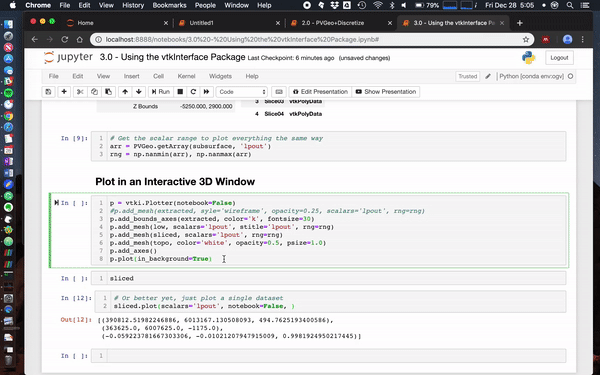
@banesullivan recently added a ton of new features to vtki (the VTK interface Python package) that help make using just about any VTK data objects more intuitive/Pythonic. If vtki is available in your Python environment then these changes make using VTK data objects way easier. Here's a screenshot of what this currently looks like in a Jupyter notebook (creates static renderings but can also be interactive in a separate pop-up window).

Also check out this notebook to see more ways to use PVGeo, discretize, and vtki. Below is a screenshot of a simple use case:

Simple example

import discretize
import numpy as np

# Create a simple TensorMesh
h1 = np.linspace(.1, .5, 3)
h2 = np.linspace(.1, .5, 5)
h3 = np.linspace(.1, .5, 3)
mesh = discretize.TensorMesh([h1, h2, h3])

# Convert to VTK object and use vtki to render it
mesh.toVTK().plot(notebook=False)

Fancy example

Here we load the Laguna del Maule Bouguer Gravity example from the SimPEG docs.

This data scene was produced from the Laguna del Maule Bouguer Gravity example provided by Craig Miller (Maule volcanic field, Chile. Refer to Miller et al 2016 EPSL for full details.)

Miller, C. A., Williams-Jones, G., Fournier, D., & Witter, J. (2017). 3D gravity inversion and thermodynamic modelling reveal properties of shallow silicic magma reservoir beneath Laguna del Maule, Chile. Earth and Planetary Science Letters, 459, 14–27. https://doi.org/10.1016/j.epsl.2016.11.007

import shelve
import tarfile
import discretize

f = discretize.utils.download(
    "https://storage.googleapis.com/simpeg/laguna_del_maule_slicer.tar.gz"
)
tar = tarfile.open(f, "r")
tar.extractall()
tar.close()

with shelve.open('./laguna_del_maule_slicer/laguna_del_maule-result') as db:
    mesh = db['mesh']
    Lpout = db['Lpout']

mesh = discretize.TensorMesh.copy(mesh)
models = {'Lpout':Lpout}
mesh.toVTK(models).plot()

Usage Notes

Since vtk and vtki are not required dependencies you'll need to make sure you install them to your Python environment. Pip install for vtki should do the trick but Windows folks might need to install vtk from conda seperately. Also this is Python 3 friendly!

pip installl vtki

Stream thickness

• from pr #95
• commits from @micmitch
• review from @lheagy

Description

Added stream_thickness keyword argument to plotSlice and _plotImage2D functions so that it is possible to scale the thickness of streamlines to reflect the amplitude of the vector field. This functionality was added in a manner similar to the stream_threshold keyword.

stream_thickness keyword currently takes a float which acts as a scaling factor for the streamline thickness. Bounds are hardwired to fix the thickness of the 10% largest and smallest vector amplitudes. Provides good results with the DC current density plots I've made but could probably be generalized in the future for more flexibility.

e.g.

mesh.plotSlice(
    u, ax=ax, normal='X', vType='F', view='vec', stream_threshold=1e-8, stream_thickness=3
)

Expand the `plot_3d_slicer` to other `vTypes` and `views`

• from pr: #121
• commits from: @prisae
• review from: @lheagy

Expand plot_3d_slicer

Addresses #116 .

Bug fix

First, it contains a minor bug-fix in the scrolling behavior (last element in each direction was not acceptable, only noticeable in small grids).

vType

Included all non-vector vType's: CC, Ex, Ey, Ez, Fx, Fy, Fz.

view

Included all view's except vec (real [default]; imag; abs; tested them all, seems to be fine).

Name-clash
There is a problem with the view-parameter, which I stupidly used to switch the x-y-axis. I changed the previous view-parameter to axis (hence axis='xy' or 'yx'). It is better to change this than to have different parameters as, for instance, in plotSlice. I added a switch for backwards-compatibility (if view in ['xy', 'yx'] => it sets axis = view; view = 'real').

Add VTK object interface

• from pr: #114
• commits from: @banesullivan
• review from: @rowanc1, @lheagy

Description

These new features enable discretize to have a direct interface for VTK base software by implementing toVTK() methods on all the mesh types (excluding CylMesh at this time). Notably, @banesullivan will be using this to provide interoperability with PVGeo to provide direct file IO into ParaView using discretize as well as ways to interactively create discretize meshes in ParaView similar to this example in the PVGeo docs. This new interface also enables discretize meshes to be passed on directly to VTK algorithms for post-processing analysis (note if you couple the interface with PVGeo like shown in this notebook, the process is somewhat simplified).

To learn more about the new VTK object interface, see the docs for the vtkInterface.

Example Usage

The VTK object interface can be used on TensorMesh, TreeMesh, and CurvilinearMesh objects to yield a VTK object in your active Python environment or used to save VTK files for easy sharing.

import discretize
import numpy as np
h1 = np.linspace(.1, .5, 3)
h2 = np.linspace(.1, .5, 5)
h3 = np.linspace(.1, .5, 3)
mesh = discretize.TensorMesh([h1, h2, h3])

# Yield a VTK data object for passing this mesh onto VTK algorithms
vtkobj = mesh.toVTK()

# Or save out the tree mesh for sharing with others
mesh.writeVTK('sample_mesh')

Note that these new features also give users the ability to specify the axes orientation of any given mesh. For example, the above TensorMesh is oriented on the traditional Cartesian reference frame by default but we could change this. To define what that orientation is, we can use the new axis_* properties:

# Defined a rotated reference frame
mesh.axis_u = (1,-1,0)
mesh.axis_v = (-1,-1,0)
mesh.axis_w = (0,0,1)
# Check that the reference frame is valid
mesh._validate_orientation()

Now we have a TensorMesh explicitly defined on a rotated reference frame! This is quite useful for when we want to convert this to a VTK data object that must have its location in a traditional XYZ Cartesian space defined.

Please take a look at the docs to learn more about using these new features!

plot_3d_slicer

• from pr #104
• commits from @prisae
• review from @lheagy

plot_3d_slicer

Add an interactive slicer for 3D volumes. At the moment only implemented for tensor meshes.

Features

• Mouse wheel scroll while hovering over a subplot scrolls through the third axis (e.g., hovering over the xy-slice and scrolling your mouse wheel will go through the z-axis).
• The three subplots are synced, also for zooming and moving.
• The initial slices can be provided via the xslice, yslice, and zslice parameters (default is in the middle of the volume).
• Transparency values and ranges can be provided (a list of floats and tuples/lists of two values), e.g. to hide the seawater or to focus on an interesting part, e.g., [0.3, [1, 4], [-np.infty, -10]] to remove all values equal to 0.3, all values between 1 and 4, and all values smaller than -10. For interactive range selection set transparency='slider'.
• Takes clim and pcolorOpts as other mesh-plotting functions, which will be passed to pcolormesh.
• By default the horizontal axis is x, and the vertical axis is y; this can be flipped by setting view='yx'.

By default, the aspect ratio of the three subplots is set to 'auto'. You can change this with the aspect
parameter, however, expect the unexpected by doing this. Most importantly, the three subplots won't be nicely aligned, and zooming might result in funny arrangements. Two parameters can be used in this respect:

• aspect takes 'auto', 'equal', or num. A list of two of them can be provided, in which case the first element is for the xy-slice, and the second element for the xz- and zy-slices. E.g., aspect=['equal', 2] sets the xy-slice to equal, and in the other two the vertical dimension is exaggerated by a factor of 2.
• The plot_3d_slicer is on a subplot2grid-grid, by default on a 3x3 grid, where 2x2 are used for the xy-slice, 2x1 for the xz-slice, and 1x2 for the zy-slice. You can provide a list of three integers via the grid-parameter, which stand for the number of grid-units occupied for the x-, y-, and z-dimension (default is [2, 2, 1]).

Usage

mesh.plot_3d_slicer(data)

It requires %matplotlib notebook in Jupyter. In regular IPython shells it should just work.

options on plotSlice, grid=True

• allow kwargs for color and linewidth in the plotgrid function
• helpful when plotting the mesh and model on a highly discretized mesh. e.g.