Car-price-prediction-ML-with-python

In this project, vehicle price estimation application was made by using machine learning algorithms.

First, we will download the libraries we will use.

! pip install category_encoders -- !pip install xgboost

import

import numpy as np # linear algebra
import pandas as pd # data processing, CSV file I/O (e.g. pd.read_csv)

# Input data files are available in the read-only "../input/" directory
# For example, running this (by clicking run or pressing Shift+Enter) will list all files under the input directory

import os
for dirname, _, filenames in os.walk('/kaggle/input'):
    for filename in filenames:
        print(os.path.join(dirname, filename))

# You can write up to 20GB to the current directory (/kaggle/working/) that gets preserved as output when you create a version using "Save & Run All" 
# You can also write temporary files to /kaggle/temp/, but they won't be saved outside of the current session

#DATA VISUALIZATION
import matplotlib.pyplot as plt
import seaborn as sns
import plotly.express as px
pd.options.mode.chained_assignment = None 
#ENCODING
import category_encoders as ce
from sklearn.preprocessing import LabelEncoder
#SCALING
from sklearn.preprocessing import StandardScaler
#Feature Selection:
from sklearn.feature_selection import VarianceThreshold
from statsmodels.stats.outliers_influence import variance_inflation_factor
from sklearn.model_selection import train_test_split
#ML
from sklearn.tree import DecisionTreeRegressor
from sklearn.ensemble import RandomForestRegressor
from sklearn.ensemble import AdaBoostRegressor
import xgboost as xg

#Metrics and Validation:
from sklearn import metrics
from sklearn.metrics import mean_squared_error
from sklearn.metrics import r2_score
from sklearn.model_selection import cross_val_score
from sklearn.model_selection import RandomizedSearchCV
from sklearn.model_selection import GridSearchCV
from sklearn.metrics import mean_absolute_error
from sklearn.metrics import mean_absolute_percentage_error

cars.head()

ncars=cars.drop_duplicates(keep=False)

ncars.head()

plt.style.use('Solarize_Light2')
plt.figure(figsize=[16,7])
for i,j in enumerate(num_col):
    plt.subplot(2,4,i+1)
    sns.boxplot(x=ncars[j])
    plt.tight_layout()
plt.show()

plt.style.use('Solarize_Light2')
plt.figure(figsize=[15,7])
for i,j in enumerate(num_col):
    plt.subplot(2,3,i+1)
    sns.boxplot(x=ccars[j])
    plt.tight_layout()
plt.show()

%matplotlib inline
for i in cat_col:
        plt.figure(figsize=[15,7])
        sns.countplot(x=ccars[i])
        plt.xticks(rotation=90)
        plt.tight_layout()
        plt.show()fig = px.treemap(data_frame=ccars,path=["Manufacturer","Category","Model"],values='Price',title='MANUFACTURER WISE TOTAL PRICE | SALES DISTRIBUTION')
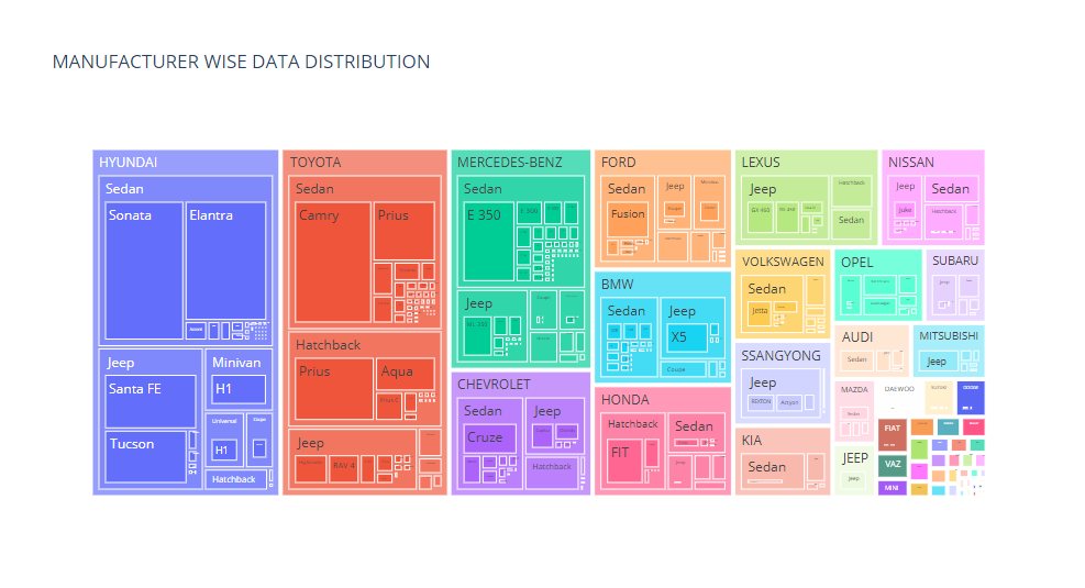
fig.show()

#To get an overview of which Category are preferred by each manufacturer
fig = px.treemap(data_frame=ccars,path=["Manufacturer","Category","Model"],title='MANUFACTURER WISE DATA DISTRIBUTION')
fig.show()

fig = px.treemap(data_frame=ccars,path=["Manufacturer","Category","Model"],values='Price',title='MANUFACTURER WISE TOTAL PRICE | SALES DISTRIBUTION')
fig.show()

Insights:

Brandwise Hyundai is the leading brand followed by Toyota and Mercedes Benz

Among cars, Jeep and Sedan type cars are most preferred by customers

Most customers wish to have leather interior for their cars

Cars with four cylinders is favourable by the customers

Most preferred fuel type:Petrol

Cars with left wheel are in higher demand

Most preferred drive wheel:front

Most preferred Gear type:Automatic

Most preferred Color:Silver,White,Grey,Black

sns.heatmap(data=ccars.corr(),cmap='YlGn',annot=True)
plt.show()

sns.pairplot(ccars[num_col])
plt.show()

#Train-Test-Split
X=ccars.copy()
X.drop(columns='Price',inplace=True)
y=ccars['Price']

cv_score_baseXGB = cross_val_score(baseXGB,X_test_ec,y_test,cv=15,scoring='r2')
print('Test Scores:',cv_score_baseXGB)

print('Score Mean',cv_score_baseXGB.mean()*100, 'Score Standard Deviation', cv_score_baseXGB.std()*100)