This project was created using R programming language.
All scripts are provided with instructions on which packages and libraries are necessary to be downloaded and used. These are also listed in the R_packages_libraries.txt file.
Important warning: do not clear the environment in R as each subsequent script relies on the dataframes produced in the previous script.
- Data_download_and_preprocess_code: R scripts for downloading data; shapefiles of watershed boundaries and .csv files of the output dataframes of the predictand and predictors for each watershed
- Model_train_and_validate_code: R script and data for formulating, fitting, and testing models for predicting evapotranspiration; .csv files of the model predictions for each watershed
- Figures_and_figure_code: markdown file showing the process of creating figures of the data and results; graphical representations of results
Each folder has their corresponding "data" folder where the outputs are stored. Each also has a readme.txt file for the instructions on how to run the scripts. Scripts are arranged and have to be run according to their sequence.
Evapotranspiration (ET) is the process of water movement from the surface of the earth to the atmosphere. It is a combination of evaporation from land surfaces and transpiration from plants and can be classified into actual (real flow of water from surface to atmosphere) and potential (demand if water availability is not restricted).
Assessing trends in evapotranspiration, a crucial component in water and energy cycles, is important in understanding and identifying changes occurring in global and local terrestrial ecosystem water balance that can be anthropogenically influenced. However, quantifying and mapping spatiotemporal distribution of ET is still a challenge and this limits the availability of accurate ET estimates necessary in making important irrigation and management decisions (Bhattarai and Wagle, 2021).
There is a wide variety of methods in estimating actual evapotranspiration using satellite-based methods and there is no consensus on which one is the best as they all come with both advantages and limitations. Remote sensing has been able to provide measurements of biophysical variables affecting evapotranspiration (i.e., albedo, vegetation type, density) and has been a cost-effective way to estimate ET, both at regional and global scales (Zhang et al., 2016). Combination of satellite data with ground measurements of actual ET and meteorological data is also another approach, making it possible to estimate ET over wide areas of varying biome types (Glenn et al., 2010). There has also been efforts in assessing trends in ET using the water balance method (i.e. subtracting the annual discharge from annual precipitation), which can be a robust approach although remains to be limited in use (Duethmann & Blöschl, 2018). For instance, a study using this approach identified that in the eastern US, ET varied systematically across climate gradient: there is a strong positive actual evapotranspiration trends in cooler regions and weak to neutral trends in warmer areas (Vadeboncoeur et al., 2018). On the other hand, an approach using a process-based ecosystem model found an increasing trend in Annual ET during 1901-2008 in the same region and that climate change determined the spatial pattern of ET changes (Yang et al., 2014). Although not in the eastern US, water balance ET can also be consistent with ET derived using energy balance models, especially in regions with water-limited ET and if interannual variability is low (Carter et al., 2018).
Findings like these are significant to various sectors and are valuable in policy making, thus, emphasizing the importance of deriving accurate ET estimates. However, in the absence of easy access to remote-sensed data, the water-balance method may be the fastest and easiest way to compute for ET. It is important to note though that this method is presented with challenges as there may be instances that there are gaps and errors in discharge and precipitation data. This therefore brings the need to establish predictive ET models that can fill in data gaps and extrapolate data and at the same time, does not require extensive data input, making it usable for water managers and decision makers.
This project aimed to develop simple regression models that can predict evapotranspiration in watersheds that represent different climatological conditions across the eastern region of US. Specifically, it sought to answer the following questions in the process of developing models:
- How does the annual actual evapotranspiration (ET) calculated using the water balance approach compare to remotely-sensed evapotranspiration?
- What are the trends in ET that are revealed by these data sets?
- Is ET dependent on the following potential controls:
- precipitation;
- atmospheric demand and energy availability (quantified through potential evapotranspiration (PET));
- soil moisture;
- average monthly maximum temperature;
- vegetation activity (Normalized Difference Vegetation Index (NDVI))?
To address these, water balance ET was computed using discharge and precipitation data and was compared to evapotranspiration derived using remote-sensed data. The potential controls were also regressed with the water balance ET to assess their effect on ET and to come up with a model that can best predict the annual total evapotranspiration in a watershed (Figure 1).
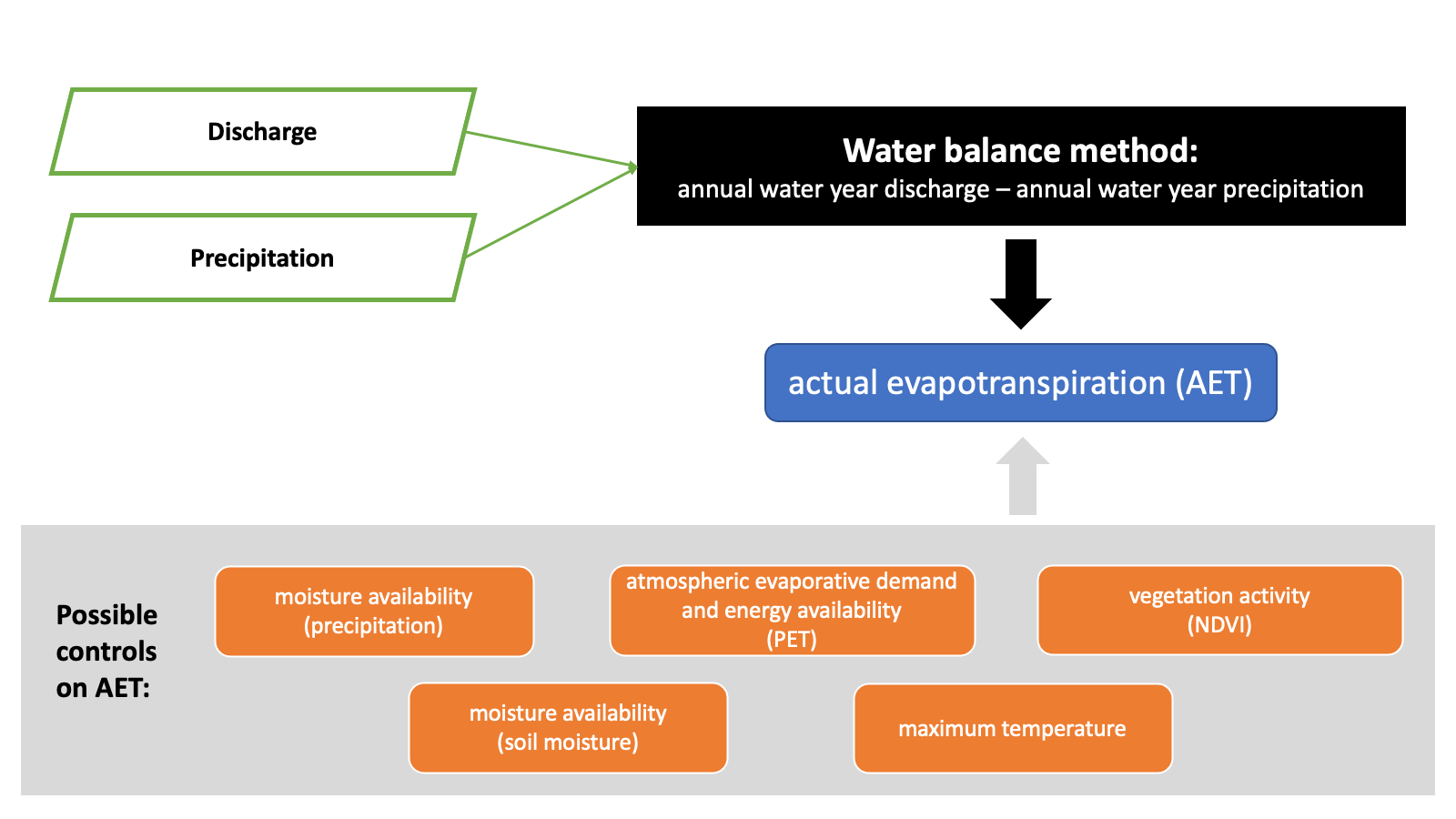 Figure 1. Conceptual framework of the study
To represent different regions in the eastern side of the continental US, the following watersheds were selected for this project:
Table 1. Selected watersheds that represent areas from north to south of US' eastern region
| Watershed | USGS Site Number | Drainage area (km2) |
|---|---|---|
| Oyster River, New Hampshire | 01073000 | 31.39 |
| Wappinger Creek, New York | 01372500 | 468.79 |
| Brandywine Creek, Pennsylvania | 01481000 | 743.33 |
| Mechums River, Virginia | 02031000 | 246.83 |
| Flat River, North Carolina | 02085500 | 385.91 |
| North Fork Edisto, South Carolina | 02173500 | 1768.96 |
| Ichawaynochaway, Georgia | 02353500 | 1605.79 |
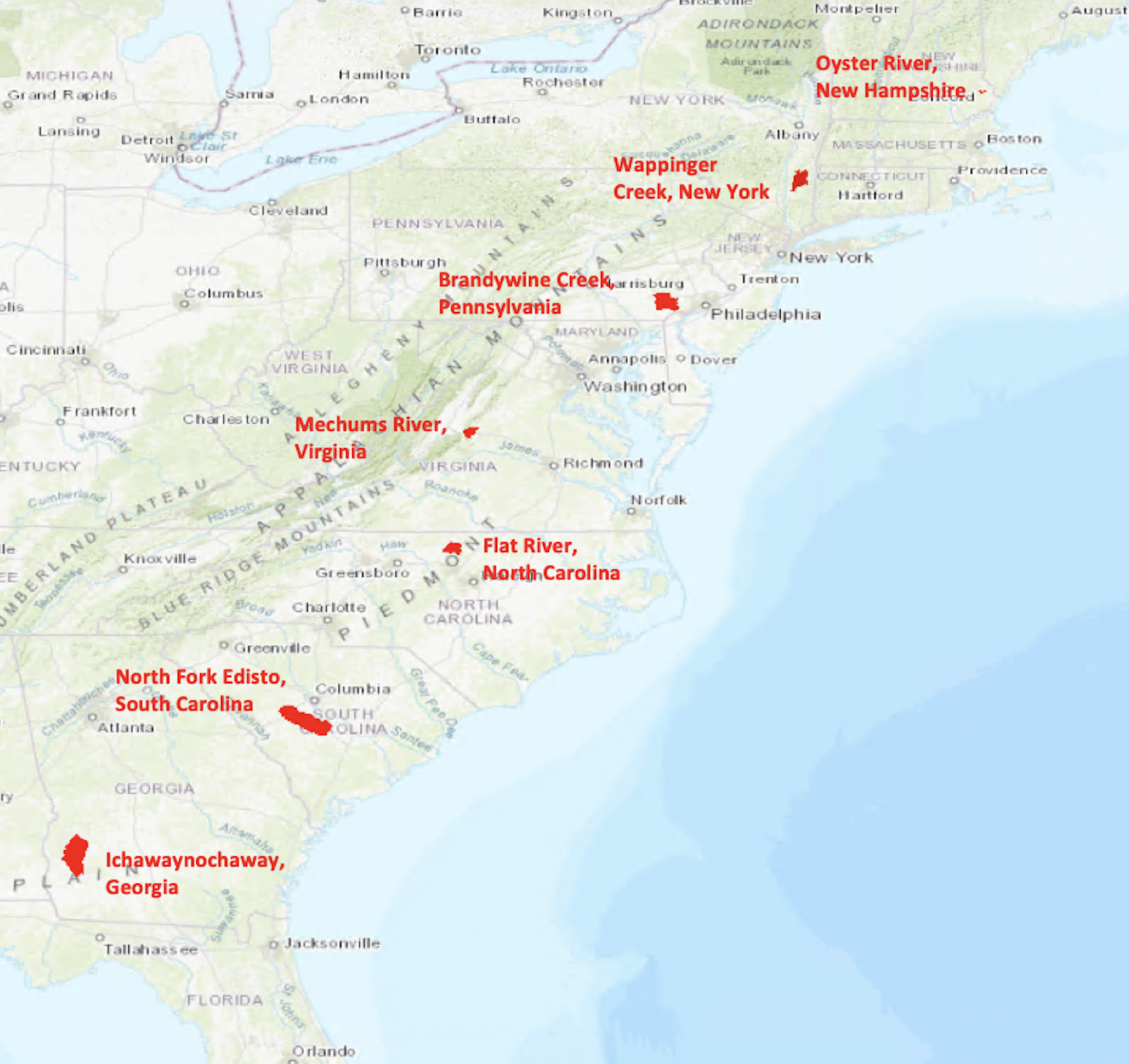
Figure 2. Location map of the watersheds
For each variable, 31 water years (1990-2020) of data were obtained. A water year is defined as the 12-month period from October 1st to September 30th of the following year (ex. October 1, 2021 to September 30, 2022 belongs to water year 2022). This is mostly used in the analysis of hydrological data to take into account that fall season is consistently the driest period and when interannual variations in storage will be the smallest. Table 2 and Figure 3 summarizes the different data that were used in this project and the corresponding R package that were used to access and download them.
To be completely based on measurements that can be done in the field unlike remote-sensed data, the variables necessary in computing for the water balance evapotranspiration used data from gauge sites:
Records of discharge from the United States Geological Survey (USGS) gauge site of each watershed were downloaded using the dataRetrieval package in R, which was created to retrieve hydrologic data from the USGS and Water Quality Portal (WQP) and load into R. With the aid of the tidyverse package, data were transformed, converted to appropriate units, and summarized per water year. The data were normalized by drainage area and expressed as basin runoff (mm).
Records of precipitation that will represent each watershed were downloaded using the rnoaa package in R, an interface to many of the National Oceanic and Atmospheric Administration (NOAA) data sources. For each of the watershed, the closest monitoring station with complete data from 1989-10-01 to 2020-09-30 was selected. Similar to the discharge data, data were transformed, converted to appropriate scale, and summarized per water year with the aid of the tidyverse package.
Given the discharge data expressed as basin runoff (mm) and the precipitation data (mm), water-balance evapotranspiration was computed by simply subtracting the annual total runoff from the annual total precipitation per water year.
In order to filter the boundaries for the remote-sensed data that would be downloaded via Google Earth Engine, the shapefile of the boundaries of each watershed were downloaded using the streamstats package in R.
For these remote-sensed predictors, the rgee package was used to access their data from Google Earth Engine using the R interface. These were all retrieved from TerraClimate: Monthly Climate and Climatic Water Balance for Global Terrestrial Surfaces, University of Idaho (Abatzoglou et al., 2018). TerraClimate provides monthly data on climatic water balance for global terrestrial surfaces at a resolution of 4638.3 meters. The data set has 14 bands corresponding to different meteorological parameters and its record covers 1958-01-01 to 2021-12-01, making it a good potential source of remote-sensed meteorological parameters that can be used to build predictive models that can fill in gaps in ground data. The actual evapotranspiration from this data set was derived using a one-dimensional soil water balance model while the PET was derived from ASCE Penman-Montieth. Likewise, soil moisture was also derived from a one-dimensional soil water balance model.
For the NDVI, two sources were used: data that covers 1989-10-01 to 2000-09-30 were obtained from Landsat 5 TM Collection 1 Tier 1 8-Day NDVI Composite (courtesy of the U.S. Geological Survey) while data that covers 2020-10-01 to 2020-09-30 were obained from MOD13A2.061 Terra Vegetation Indices 16-Day Global 1km. Both image collections have a band corresponding to the NDVI which were extracted using the rgee package in R.
For all the remote-sensed data, the tidyverse package was used to transform them and make necessary scaling prior to summarizing them per water year. A final data frame for each watershed consisting the predictand and predictors were created and exported as .csv files.
Table 2. Sources of other data used in this project and the corresponding R package available to download them
| Data | Source/Description | R package | URL |
|---|---|---|---|
| discharge | United States Geological Survey (USGS) | dataRetrieval | https://cran.r-project.org/web/packages/dataRetrieval/vignettes/dataRetrieval.html |
| precipitation (gauge) | National Oceanic and Atmospheric Administration (NOAA) | rnoaa | https://cran.r-project.org/web/packages/rnoaa/index.html |
| watershed boundary | United States Geological Survey (USGS) | streamstats | https://github.com/markwh/streamstats |
| evapotranspiration | TerraClimate: Monthly Climate and Climatic Water Balance for Global Terrestrial Surfaces, University of Idaho | https://developers.google.com/earth-engine/datasets/catalog/IDAHO_EPSCOR_TERRACLIMATE | |
| potential evapotranspiration, precipitation (gridded), soil moisture, monthly maximum temperature | ^ | rgee | https://github.com/r-spatial/rgee |
| NDVI | Landsat 5 TM Collection 1 Tier 1 8-Day NDVI Composite | ^ | https://developers.google.com/earth-engine/datasets/catalog/LANDSAT_LT05_C01_T1_8DAY_NDVI#description |
| ^ | MOD13A2.061 Terra Vegetation Indices 16-Day Global 1km | ^ | https://developers.google.com/earth-engine/datasets/catalog/MODIS_061_MOD13A2#description |
Following the process of supervised learning (VanderPlas, 2016) and to evaluate the roles of the potential controls on evapotranspiration, a multiple linear regression relationship was fit between these predictors and the annual water balance ET for each site using the equation:
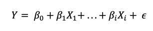
where Y is the dependent variable (water-balance ET); β0 is the intercept; βi is the slope of the Xi independent variables; and ϵ is the model's error term.
Prior to making the regression models, the final dataframe from the previous step which contains 31 water years of the water-balance ET and the predictors were divided into training and validation data set (1990-2013, 25 years) for fitting the model and 20% of the data (2014-2020, 7 years) were separated and not processed for use in testing and evaluation of the model fit.
For each watershed, the data set was inspected for multicollinearity by making a correlation plot and checking the corrrelation values between predictors. A threshold of | > 0.7 | was used to determine if variables have high correlation or not. Regression models were created using the lm() function from the stats package in R. Initially, a model with all the predictor variables and a model with single predictor variable (precipitation, based on its consistent good linear relationship with the water balance ET) were made. The vif() function from the car package was used to check for the Variance Inflation Factor (VIF) of the model's parameters in order to detect multicollinearity.
To check model performance, the adjusted R2 and p-values of the model and each variable in it were considered. Subset regression using leaps, which identifies the best combination of variables that will give the highest adjusted R2, was used to create models. To further aid in identifying the "best" model, stepwise regression using an F test using MASS and stepAIC were also done. The AIC and BIC of each model were also assessed. In the end, the goal was to select a model that gives the highest adjusted R2 with, as much as possible, all variables significant at alpha = 0.05 level. The final model also should not have multicollinear variables.
The selected "best" model was also checked for violations of ordinary least squares assumptions by inspecting plots of predictions versus residuals, observed values versus predicted values, and model residuals and predicted values. The model's residuals were also tested for normality using probability plot correlation test statistic (also known as Ryan Joiner test for normality which computes for Blom's plotting position) and Shapiro-Wilk test for normality using the shapiro.test() from the base stats package in R. Autocorrelation among the residuals were also checked using the acf() function. After confirming that the selected model's residuals are normal, this was used to predict for the ET using the training data set and the testing data set.
In order to compare the water balance ET and remote-sensed ET, normality and equality of variances of the data were checked first using shapiro.test() and var.test() functions, respectively. An independent samples test was then done using t.test() to determine if the means of the two data sets are significantly different.
Graphical representations of the predictors and models were created using the ggplot2 package.
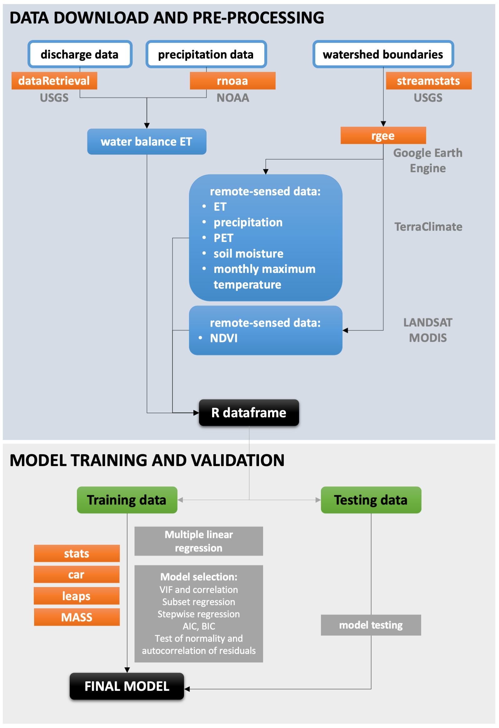 Figure 3. Methodological framework of the study. Important R packages used are in the orange rectangles.
Trends in the predictor variables, particularly for annual total potential evapotranspiration and average monthly maximum temperature show the expected difference in the climatic profile among the watersheds depending on their location (i.e., higher PET and temperature at watersheds in lower latitude). It is important to note that for NDVI, while the trend is consistent (higher NDVI at watersheds in higher latitude), the values coming from LANDSAT differ by approximately less than 0.1 compared to the values that come from MODIS. This gap is even wider among annual average NDVI, hence, the decision to use the maximum NDVI instead in the regression analysis (Figure 4).
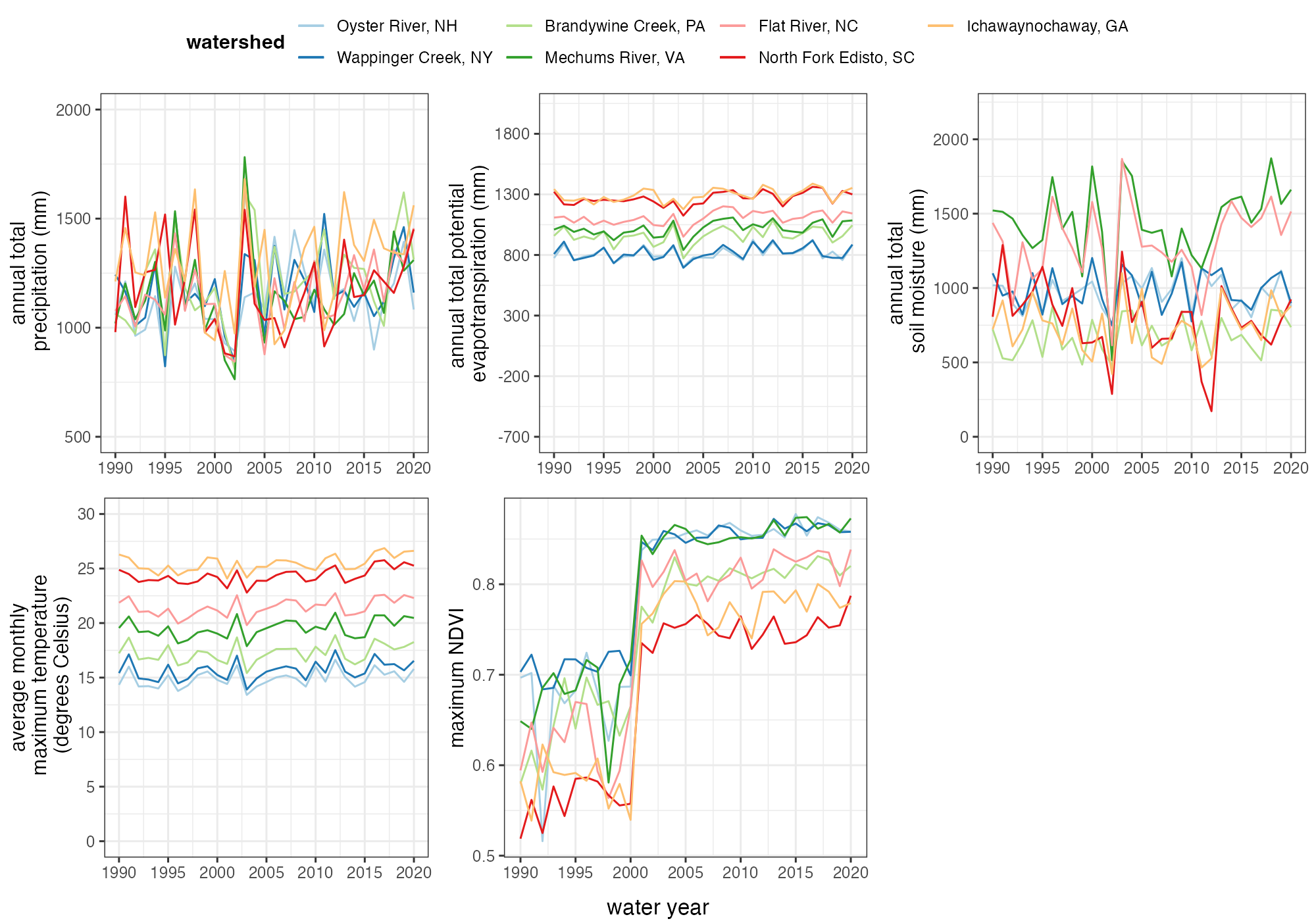 Figure 4. Annual total precipitation, total potential evapotranspiration, total soil moisture, average monthly maximum temperature, and maximum NDVI from water years 1990-2020
The computed evapotranspiration using water balance method in some of the watersheds (Oyster River, NH and Wappinger Creek, NY) yielded negative values, which can potentially be due to discrepancies in the precipitation and discharge data. These negative values were omitted from the data prior to making the models as they do not accurately represent expected evapotranspiration values. Most of the computed water balance evapotranspiration reveal a slight increase in trend from water year 1990 to 2020 (Figure 5). The average annual water balance ET ranges from 505 to 943 mm, with the lowest in Wappinger Creek, NY and the highest in North Fork Edisto, SC.
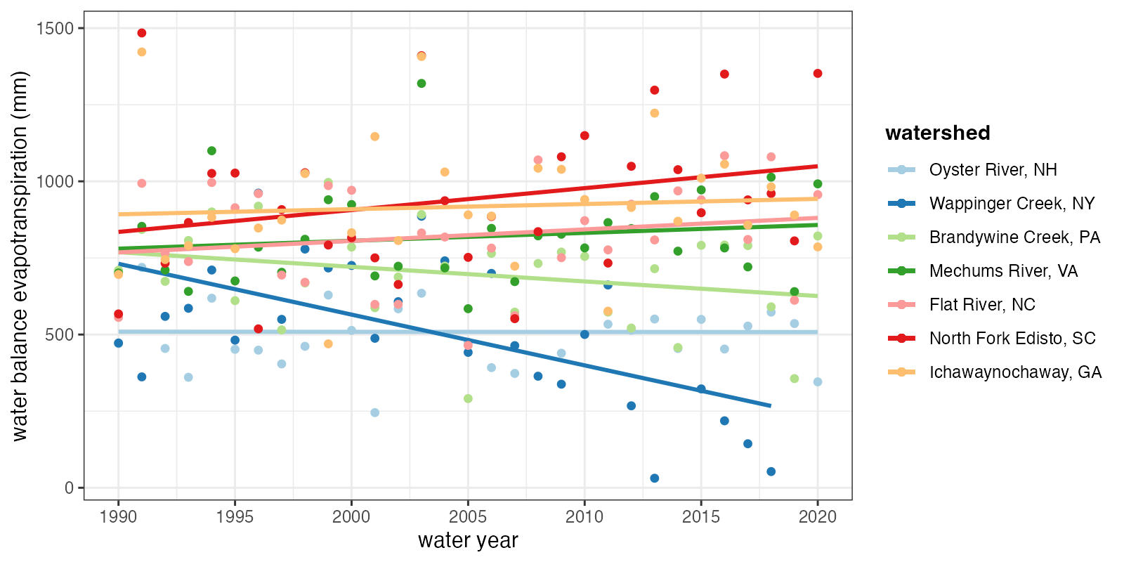 Figure 5. Annual evapotranspiration from water years 1990-2020 computed using water balance method
Comparison of water balance ET with remote-sensed ET shows a more steady trend across the record in the remote-sensed data compared to high variations in the water-balance derived data (Figure 6). Test for equality of variances between the two data sets among all watersheds indicate that their variances are not equal, with the ratio ranging from 0.03 to 0.11 (i.e. ratio closer to 1 indicates closer similarity in variance). On the other hand, t-test of their means indicate that in all watersheds, the means of the water-balance ET and the remote-sensed ET are significantly different. This indicate that the two data sets are highly different.
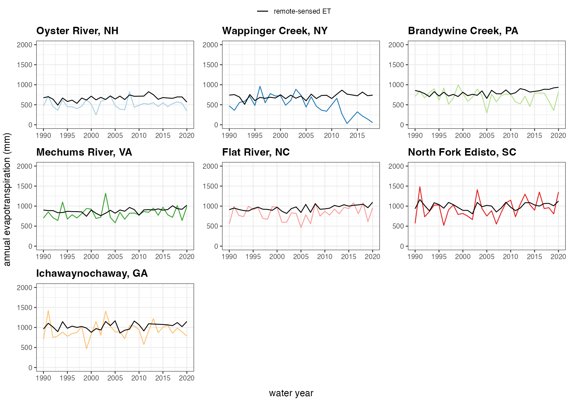 Figure 6. Comparison of evapotranspiration computed using water balance method and evapotranspiration from remote-sensed data
Multiple linear regression of all predictor variables with the water balance ET indicate the significance of precipitation to be included in predictive models (Table 3). This is further confirmed among the “best” models selected for each watershed (Table 4), wherein precipitation is consistently included and a significant variable in the model. Precipitation also shows the similar trend with water-balance evapotranspiration (Figure 7). On the other hand, PET and monthly maximum temperature are also consistently highly collinear, which can be expected since the PET from TerraClimate was derived using ASCE Penman-Monteith model, which uses air temperature in its equation, and at the same time, higher temperatures are known to increase rate of evaporation.
Adjusted R2 ranged from 0.1013 to 0.7695, with the model for Oyster River, NH that includes precipitation and PET performing most poorly and the model for North Fork Edisto, SC that includes precipitation and NDVI performing the "best".
Table 3. Predictor variables and their corresponding coefficient estimates and p-values in multiple linear regression model wherein all predictors are regressed against the water-balance evapotranspiration. Cells in light blue are the variables that are significant at alpha = 0.05
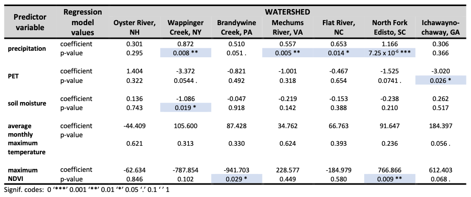
Table 4. Final regression model of each watershed
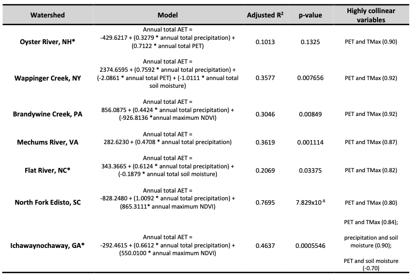
* Only precipitation is the significant variable
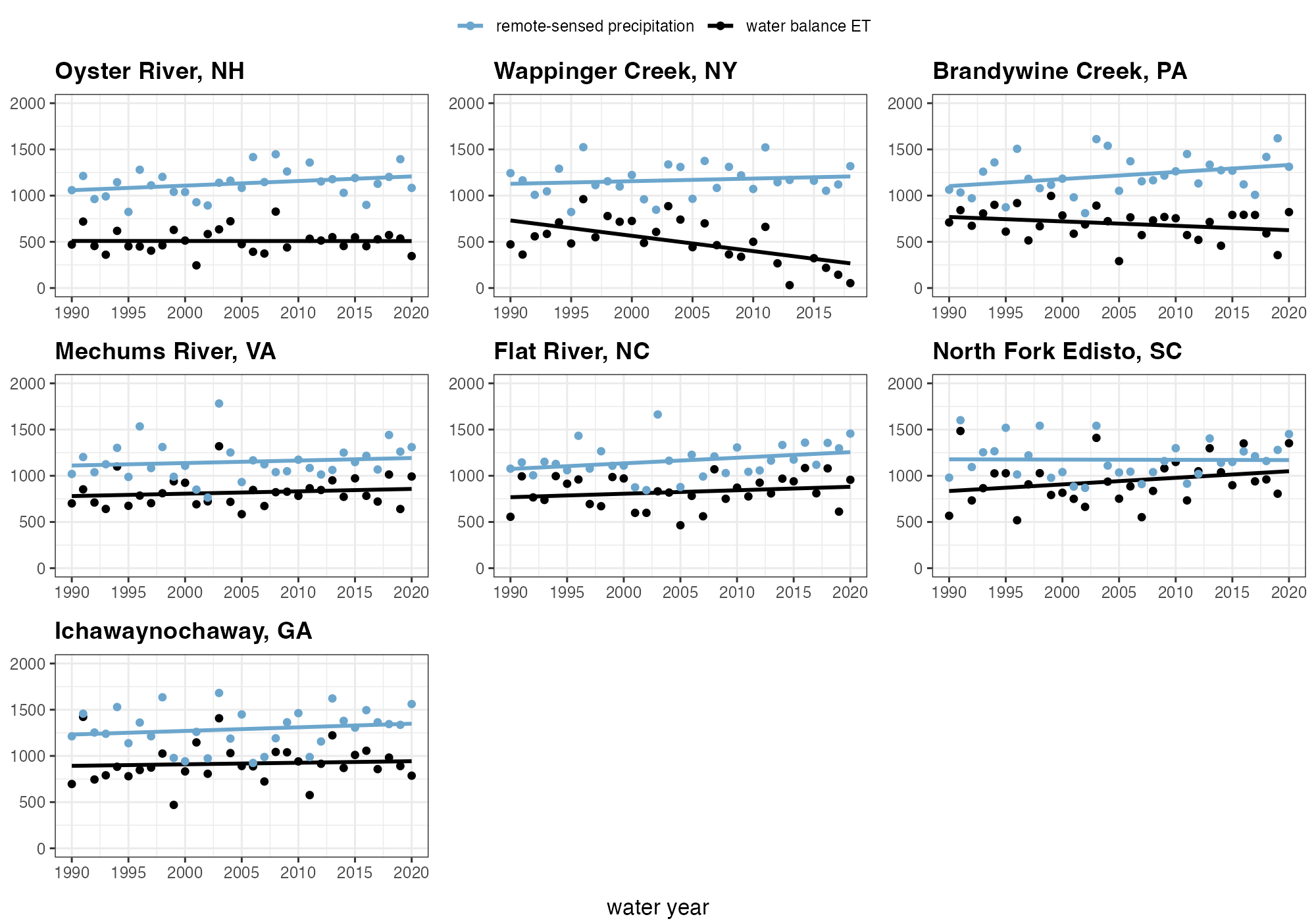 Figure 7. Trends in remote-sensed precipitation and water-balance evapotranspiration.
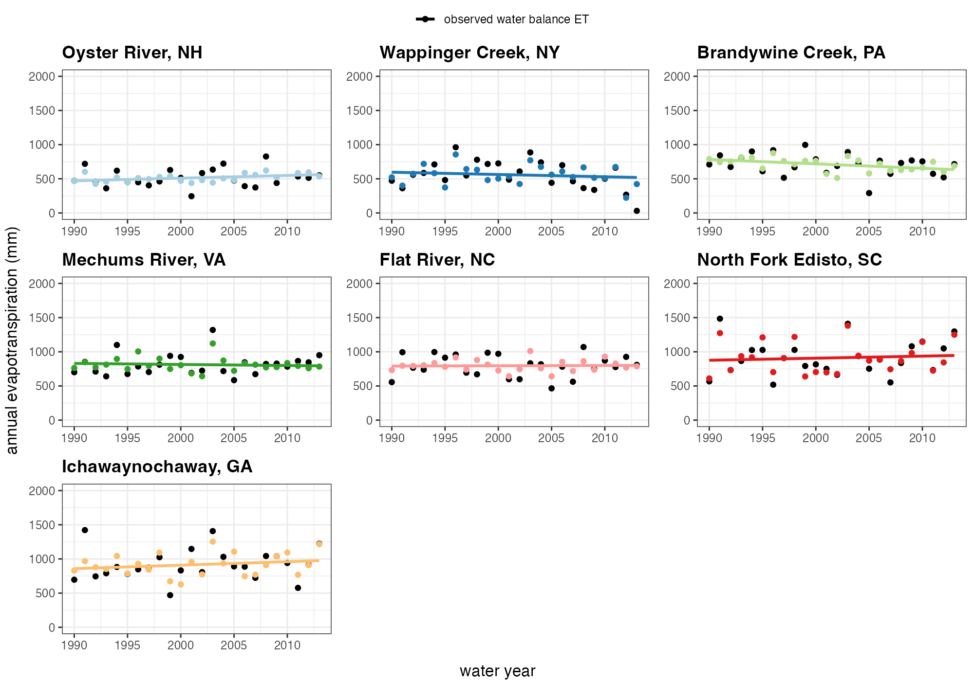 Figure 8. Predicted versus observed (water balance) annual evapotranspiration. Points in black are the computed water balance ET while points in color are the predicted values using the "best" regression model for each watershed.
The evapotranspiration derived from water balance method is significantly different from the evapotranspiration derived from remote-sensed data. Since the water balance ET computed for this project was limited to data from one discharge and one precipitation gauge site, it may be inappropriate to compare the two data sets as the method employed already misses out variations across the entire watershed that may improve the estimate. On the other hand, remote-sensed data from TerraClimate may also have its limitations as stated in their Google Earth Engine catalog: data is inherited from parent datasets, do not capture temporal variability at finer scales than parent datasets, and the water balance model used is very simple and does not account for heteregeneity in vegetation types. Nonetheless, the absence of big peaks/lows and data jumps in the remote-sensed ET (Figure 6) suggests that it can be a more reliable estimate of evapotranspiration. It is also important to note that water balance estimates are not direct measurements and may be affected by other aspects of the water budget (Vadeboncoeur et al., 2018).
The variables included in the "best" model for each watershed varies but precipitation is consistently a significant predictor. This can be expected since precipitation provides the water and moisture and ET generally uses a large fraction of this. Other than precipitation, PET, soil moisture, and NDVI also aided in improving a model's performance, hence, suggesting their importance in explaning variabilities in ET. The model with the highest adjusted R2 is for the North Fork Edisto, SC watershed, which includes precipitation and NDVI among its predictor variables. Aside from precipitation, NDVI can also be a good predictor since it represents vegetation activity within the watershed. Dense vegetation (high NDVI) indicates larger surface area available for transpiration to occur, hence, affecting annual evapotranspiration measurements. Again, since accuracy in the water balance ET that is used as the dependent variable in the regression models is potentially low, these models may not really be fully representing the drivers of ET variability in these watersheds. In addition, regression relationships may not also be fully revealing real physical relationships. Results of this project emphasize the importance of using high quality data sets of discharge, precipitation, and other climate variables.
This project analyzed the difference between evapotranspiration derived using the water balance equation versus remote-sensed data, as well as its potential controls among the available meteorological parameters from an extensive remote-sensed data set, particularly precipitation, PET, soil moisture, maximum temperature, and NDVI. This was to come up with a model that can rely on available remote-sensed data to fill in gaps in ground data, as well as to identify drivers of ET. Annual water balance ET was found to be significantly different from annual remote-sensed ET across all watersheds. Consistently, precipitation was found to be an important predictor across all the "best" models from each watershed. While model residuals are normal, poor adjusted R2 values indicate that the included variables are not explaining variations in ET very well. In addition, this suggest that other more important parameters that were not explored could be missing in the models to make them better at predicting ET.
The results of this study is highly limited by the quality of the data that were obtained. Moving forward, the following can be done to improve the entire project:
- improving the computed water balance ET by using data from multiple gauge sites within the watershed instead of relying on stations at or close to the outlet;
- quality check on the downloaded remote-sensed data and exploration of other data sets other than TerraClimate;
- extending data length in order to improve training and testing data for regression models.
Bhattarai, N., & Wagle, P. (2021). Recent Advances in Remote Sensing of Evapotranspiration. Remote Sensing, 13(21), 4260. https://doi.org/10.3390/rs13214260
Carter, E., Hain, C., Anderson, M., & Steinschneider, S. (2018). A Water Balance–Based, Spatiotemporal Evaluation of Terrestrial Evapotranspiration Products across the Contiguous United States. Journal of Hydrometeorology, 19(5), 891–905. https://doi.org/10.1175/JHM-D-17-0186.1
Duethmann, D., & Blöschl, G. (2018). Why has catchment evaporation increased in the past 40 years? A data-based study in Austria. Hydrology and Earth System Sciences, 22(10), 5143–5158. https://doi.org/10.5194/hess-22-5143-2018
Glenn, E. P., Nagler, P. L., & Huete, A. R. (2010). Vegetation Index Methods for Estimating Evapotranspiration by Remote Sensing. Surveys in Geophysics, 31(6), 531–555. https://doi.org/10.1007/s10712-010-9102-2
Vadeboncoeur, M. A., Green, M. B., Asbjornsen, H., Campbell, J. L., Adams, M. B., Boyer, E. W., Burns, D. A., Fernandez, I. J., Mitchell, M. J., & Shanley, J. B. (2018). Systematic variation in evapotranspiration trends and drivers across the Northeastern United States. Hydrological Processes, 32(23), 3547–3560. https://doi.org/10.1002/hyp.13278
VanderPlas, J. (2016, November). What Is Machine Learning? | Python Data Science Handbook. https://jakevdp.github.io/PythonDataScienceHandbook/05.01-what-is-machine-learning.html
Yang, Q., Tian, H., Li, X., Tao, B., Ren, W., Chen, G., Lu, C., Yang, J., Pan, S., Banger, K., & Zhang, B. (2015). Spatiotemporal patterns of evapotranspiration along the North American east coast as influenced by multiple environmental changes. Ecohydrology, 8(4), 714–725. https://doi.org/10.1002/eco.1538
Zhang, K., Kimball, J. S., & Running, S. W. (2016). A review of remote sensing based actual evapotranspiration estimation. WIREs Water, 3(6), 834–853. https://doi.org/10.1002/wat2.1168
Abatzoglou, J.T., S.Z. Dobrowski, S.A. Parks, K.C. Hegewisch, 2018, Terraclimate, a high-resolution global dataset of monthly climate and climatic water balance from 1958-2015, Scientific Data 5:170191, doi:10.1038/sdata.2017.191
MOD13A2 v061. https://doi.org/10.5067/MODIS/MOD13A2.061
Aybar C (2022). rgee: R Bindings for Calling the 'Earth Engine' API. R package version 1.1.5, https://CRAN.R-project.org/package=rgee.
Chamberlain S (2021). rnoaa: 'NOAA' Weather Data from R. R package version 1.3.8, https://CRAN.R-project.org/package=rnoaa.
De Cicco, L.A., Hirsch, R.M., Lorenz, D., Watkins, W.D., 2022, dataRetrieval: R packages for discovering and retrieving water data available from Federal hydrologic web services, v.2.7.11, doi:10.5066/P9X4L3GE
Garrett Grolemund, Hadley Wickham (2011). Dates and Times Made Easy with lubridate. Journal of Statistical Software, 40(3), 1-25. URL https://www.jstatsoft.org/v40/i03/.
Hagemann M (2022). streamstats: R bindings to the USGS Streamstats API. R package version 0.0.3.
Henry L, Wickham H (2022). purrr: Functional Programming Tools. R package version 0.3.5, https://CRAN.R-project.org/package=purrr.
Fox, J. and Weisberg, S. (2019). An {R} Companion to Applied Regression, Third Edition. Thousand Oaks CA: Sage. URL: https://socialsciences.mcmaster.ca/jfox/Books/Companion/
Kassambara A (2022). ggpubr: 'ggplot2' Based Publication Ready Plots. R package version 0.5.0, https://CRAN.R-project.org/package=ggpubr.
Miller TLboFcbA (2020). leaps: Regression Subset Selection. R package version 3.1, https://CRAN.R-project.org/package=leaps.
Müller K, Wickham H (2022). tibble: Simple Data Frames. R package version 3.1.8, https://CRAN.R-project.org/package=tibble.
Pebesma, E., 2018. Simple Features for R: Standardized Support for Spatial Vector Data. The R Journal 10 (1), 439-446, https://doi.org/10.32614/RJ-2018-009
R Core Team (2022). R: A language and environment for statistical computing. R Foundation for Statistical Computing, Vienna, Austria. URL https://www.R-project.org/.
Spinu V (2022). timechange: Efficient Manipulation of Date-Times. R package version 0.1.1, https://CRAN.R-project.org/package=timechange.
Venables, W. N. & Ripley, B. D. (2002) Modern Applied Statistics with S. Fourth Edition. Springer, New York. ISBN 0-387-95457-0
Wickham H, François R, Henry L, Müller K (2022). dplyr: A Grammar of Data Manipulation. R package version 1.0.10, https://CRAN.R-project.org/package=dplyr.
Wickham H (2022). forcats: Tools for Working with Categorical Variables (Factors). R package version 0.5.2, https://CRAN.R-project.org/package=forcats.
Wickham H. ggplot2: Elegant Graphics for Data Analysis. Springer-Verlag New York, 2016.
Wickham H, Hester J, Bryan J (2022). readr: Read Rectangular Text Data. R package version 2.1.3, https://CRAN.R-project.org/package=readr.
Wickham H (2022). stringr: Simple, Consistent Wrappers for Common String Operations. R package version 1.4.1, https://CRAN.R-project.org/package=stringr.
Wickham H, Girlich M (2022). tidyr: Tidy Messy Data. R package version 1.2.1, https://CRAN.R-project.org/package=tidyr.