ResDAG

Reservoir computing for PyTorch.
Compose reservoir models as DAGs, train readouts with a single algebraic solve, run it all on the GPU.

---

ResDAG treats reservoir models — echo state networks and beyond — as ordinary PyTorch layers. Reservoirs, readouts, and transforms are nn.Modules wired together with a functional API; training a readout is one teacher-forced pass and one algebraic ridge solve, with no epochs. Models move with .to(device), serialize with state_dict(), and embed in larger PyTorch pipelines, optimizers included.

Documentation →

Installation

pip install resdag            # core
pip install "resdag[hpo]"     # + Optuna hyperparameter optimization

Python ≥ 3.11, PyTorch ≥ 2.10.

Docs track the dev branch. Releases are frozen until 1.0, so PyPI serves 0.6.2 — which predates parts of the documented API (the ESN facade, resdag.data streaming, the newer readout solvers). For the documented API today: pip install "git+https://github.com/El3ssar/ResDAG".

Try it

A reservoir forecaster on a toy signal, end to end:

import torch
import resdag as rd

t = torch.linspace(0, 60, 3000)
data = torch.sin(t).reshape(1, -1, 1)            # (batch, time, features)

warmup, train, target, f_warmup, val = rd.utils.prepare_esn_data(
    data, warmup_steps=100, train_steps=2000, val_steps=300)

model = rd.models.classic_esn(reservoir_size=300, feedback_size=1, output_size=1)
rd.ESNTrainer(model).fit((warmup,), (train,), targets={"output": target})

prediction = model.forecast(f_warmup, horizon=300)   # autoregressive, (1, 300, 1)

The first forecast walkthrough does the same on the Lorenz attractor, with the math explained.

Compose, don't configure

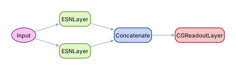
Architectures are DAGs you wire, not options you toggle. Two reservoirs on different timescales, read out together:

from resdag import CGReadoutLayer, Concatenate, ESNModel, reservoir_input
from resdag.layers import ESNLayer

inp    = reservoir_input(3)
fast   = ESNLayer(64, feedback_size=3, leak_rate=1.0, spectral_radius=0.9)(inp)
slow   = ESNLayer(64, feedback_size=3, leak_rate=0.2, spectral_radius=0.9)(inp)
merged = Concatenate()(fast, slow)
model  = ESNModel(inp, CGReadoutLayer(128, 3, name="output")(merged))

Branches, feature augmentations, and multiple readout heads compose the same way — one reservoir, squared-state augmentation, two heads:

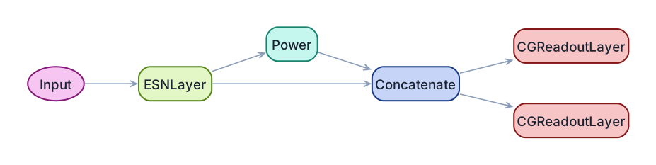
All heads fit in a single pass, in dependency order. The composition handbook covers the patterns.

Coming from scikit-learn?

The whole fit → predict loop fits in one object. ESN.fit(series) slices the warmup window, builds the one-step-ahead target, and runs the algebraic solve; forecast(horizon=...) re-synchronizes and rolls out — numpy in, numpy out:

import numpy as np
from resdag import ESN

series = np.cumsum(np.random.randn(2000, 3), axis=0)   # (time, features)

esn = ESN(reservoir_size=300, spectral_radius=0.9).fit(series)
prediction = esn.forecast(horizon=200)                 # (200, 3)

esn.model drops you back into the full composable graph whenever you outgrow the facade. The mental model maps fit/predict onto ResDAG's warmup + ESNTrainer.fit / forecast flow.

Train through it with SGD

A reservoir is an ordinary PyTorch layer, so it drops into a pipeline as a frozen feature extractor and you train any head with a normal optimizer loop. The reservoir has zero trainable parameters, so the optimizer only ever touches the head:

import torch
import torch.nn as nn
from resdag import ReservoirFeatureExtractor

net = nn.Sequential(
    ReservoirFeatureExtractor(500, feedback_size=3, spectral_radius=0.9),
    nn.Linear(500, 64), nn.Tanh(), nn.Linear(64, n_classes),
)
extractor, head = net[0], net[1:]
opt = torch.optim.Adam(head.parameters(), lr=1e-3)     # head only — reservoir is frozen

with torch.no_grad():                                  # frozen features: compute once
    extractor.on_epoch_start()
    feats = extractor(sequences)[:, -1]                # (batch, 500) last-step summary

for _ in range(300):
    loss = nn.functional.cross_entropy(head(feats), labels)
    opt.zero_grad(); loss.backward(); opt.step()

This is the pure-PyTorch path: gradient heads, full BPTT through the recurrence (trainable=True), and embedding frozen reservoirs in larger networks. Work · Train covers all three training paths; Work · Scale & deploy shows the frozen-backbone classifier inside a nn.Module pipeline.

Documentation

Start	Install, a first trained forecaster, the mental model
Build	Layers, readouts, architectures, topologies, initializers
Work	Training paths, forecasting with drivers, tuning, GPU
Theory	Every equation, stated against the code
Reference	The full public API

Ecosystem

Built on pytorch_symbolic for graph composition. Pairs with TSDynamics, a companion library of dynamical systems — it generates the systems, ResDAG forecasts them.

Contributing

See CONTRIBUTING.md — releases are automated from conventional commits, and most component types are one registry decorator away.

License

MIT — © Daniel Estevez-Moya