
'mispitools' is an open-source package written in the R statistical language. It consists of a collection of decision-making tools designed for conducting missing person searches. The package enables the computation of various features, ranging from non-genetic data based likelihood ratios (LRs) to the optimal LR threshold for identifying potential matches in database searches. Examples of non-genetic data are: biological sex, pigmentation traits, age, among others.
To properly cite 'mispitools,' please use the following references:
- Marsico et al., Forensic Science International: Genetics, 2023 (https://doi.org/10.1016/j.fsigen.2023.102891)
- Marsico et al., Forensic Science International: Genetics, 2021 (https://doi.org/10.1016/j.fsigen.2021.102519)
Additionally, an add-on package draft is under construction, and it can be useful for a deeper introduction to the package:
- Marsico, BioRxiv 2024 (https://doi.org/10.1101/2024.08.16.608307)
'mispitools' imports two additional packages, namely forrel (https://doi.org/10.1016/j.fsigen.2020.102376) and pedtools (https://doi.org/10.1016/C2020-0-01956-0).
The objective of mispitools is to provide a simulation framework for decision-making in missing person identification cases. You can install it from CRAN by typing the following command on R:
install.packages("mispitools")
library(mispitools)
You can also install the unstable versions of mispitools from Github by using the following command:
install.packages("devtools")
library(devtools)
install_github("MarsicoFL/mispitools")
Now you can analyze the mispitools documentation, which provides descriptions for all functions and parameters.
?mispitoolsNOTE: These packages should be installed automatically as dependencies with mispitools. However, in some cases, it may be necessary to install them manually, especially if you are installing the development version from GitHub. You can do this by using the following lines:
install.packages("ggplot2")
install.packages("forrel")
install.packages("pedtools")
install.packages("reshape2")
install.packages("tidyverse")
install.packages("patchwork")NOTE: The methodology implemented in this section is explained in: https://doi.org/10.1016/j.fsigen.2023.102891 (or the open pre-print version, available on http://dx.doi.org/10.2139/ssrn.4331033).
Now you are able to compute conditional probability phenotype tables considering the variables Age, Sex, and Hair color. Firstly, you can analyze the different parameters from the documentation.
?CPT_POPFor simplification, the population reference age distribution is assumed to be uniform. However, the function can be easily adapted to incorporate a dataset with the specified frequencies. This feature will be implemented in the near future.
CPT_POP(
  propS = c(0.5, 0.5),
  MPa = 40,
  MPr = 6,
  propC = c(0.3, 0.2, 0.25, 0.15, 0.1))
## [,1] [,2] [,3] [,4] [,5]
## F-T1 0.0225 0.015 0.01875 0.01125 0.0075
## F-T0 0.1275 0.085 0.10625 0.06375 0.0425
## M-T1 0.0225 0.015 0.01875 0.01125 0.0075
## M-T0 0.1275 0.085 0.10625 0.06375 0.0425
The obtained matrix represents the probabilities of the phenotypes in the reference population. F-T1 represents a female whose age matches with the age of the missing person. F-T0 represents a female with a mismatch in age with the missing person. M-T1 and M-T0 correspond to the same age categories in association with male. The numbers (columns) represent different hair colors. It is important to note that in the following case, the parameters remain the same, but changing the MP (missing person) range will alter the population probabilities.
CPT_POP(
  propS = c(0.5, 0.5),
  MPa = 40,
  MPr = 15,
  propC = c(0.3, 0.2, 0.25, 0.15, 0.1))
## [,1] [,2] [,3] [,4] [,5]
## F-T1 0.05625 0.0375 0.046875 0.028125 0.01875
## F-T0 0.09375 0.0625 0.078125 0.046875 0.03125
## M-T1 0.05625 0.0375 0.046875 0.028125 0.01875
## M-T0 0.09375 0.0625 0.078125 0.046875 0.03125
This can be counterintuitive because the population frequencies remain the same in both cases. However, the values of T1 and T0 depend on the age of the missing person (MP) and the error rate. Similarly, it is possible to compute MP conditioned probabilities. Once again, I recommend referring to the documentation for more details on this process.
?CPT_MPThen, we can select a specific missing person (MP). One of the parameters is epc, which is derived from the function Cmodel(). Let's take a look at that function:
?Cmodel()The Cmodel() function provides two options: "uniform" and "custom". The "uniform" option assigns the same error probability (ep) for all combinations of colors, while the "custom" option allows you to specify a specific value for each pair. In this case, we will select the "custom" option.
Cmodel(
  errorModel = "custom",
  ep = 0.01,ep12 = 0.01,ep13 = 0.005,
  ep14 = 0.01,ep15 = 0.003,ep23 = 0.01,
  ep24 = 0.003,ep25 = 0.01,ep34 = 0.003,
  ep35 = 0.003,ep45 = 0.01)
## [,1] [,2] [,3] [,4] [,5]
## [1,] 0.972762646 0.009727626 0.004863813 0.009727626 0.002918288
## [2,] 0.009680542 0.968054211 0.004840271 0.009680542 0.002904163
## [3,] 0.004897160 0.009794319 0.979431929 0.002938296 0.002938296
## [4,] 0.009746589 0.002923977 0.002923977 0.974658869 0.009746589
## [5,] 0.002923977 0.009746589 0.002923977 0.009746589 0.974658869
Now we can specify the phenotype probabilities conditioned on the characteristics of the missing person (MP).
CPT_MP(MPs = "F", MPc = 1,
       eps = 0.05, epa = 0.05,
       epc = Cmodel())
## 1 2 3 4 5
## F-T1 0.877918288 8.779183e-03 4.389591e-03 8.779183e-03 2.633755e-03
## F-T0 0.046206226 4.620623e-04 2.310311e-04 4.620623e-04 1.386187e-04
## M-T1 0.046206226 4.620623e-04 2.310311e-04 4.620623e-04 1.386187e-04
## M-T0 0.002431907 2.431907e-05 1.215953e-05 2.431907e-05 7.295720e-06
Moreover, LR can be computed as follows:
MP <- CPT_MP(MPs = "F", MPc = 1,
       eps = 0.05, epa = 0.05,
       epc = Cmodel())
POP <- CPT_POP(
  propS = c(0.5, 0.5),
  MPa = 40,
  MPr = 6,
  propC = c(0.3, 0.2, 0.25, 0.15, 0.1))

MP/POP
## 1 2 3 4 5
## F-T1 39.01859058 0.5852788586 0.2341115435 0.7803718115 0.351167315
## F-T0 0.36240177 0.0054360266 0.0021744106 0.0072480354 0.003261616
## M-T1 2.05361003 0.0308041505 0.0123216602 0.0410722006 0.018482490
## M-T0 0.01907378 0.0002861067 0.0001144427 0.0003814755 0.000171664
We can see that the sex-age-color: F-T1-1 and M-T1-1 are the only two LR values over 1, being the former (perfect match) the largest. All these information could be summarized in the following plot:
library(ggplot2)
CondPlot(POP,MP)
Furthermore, a ShinyApp could be executed using the following command:
mispiApp()It will open an interactive panel where you can select parameters to compute conditioned probability tables and likelihood ratios (LR) for each phenotype. The parameter "PropF" represents the proportion of females in the population, and the male proportion is calculated as 1 minus PropF. "PropC" indicates the proportion of a specific hair color. After defining proportions for five hair colors, mispitools normalizes them so that they sum up to 1.

Note: mispiApp is currently under development. Specifically, the age variable assumes a uniform population frequency distribution from 0 to 80 years old. Introducing inconsistent parameters, such as setting MPa (missing person age) to 40 with a range error (MPr) of 100 (an error that exceeds two times the age and allows negative results), will result in inconsistent probabilities. Please ensure that you select reliable values for accurate calculations.
NOTE: The methodology used in this section is explained in: https://doi.org/10.1016/j.fsigen.2021.102519
In this example, forrel and pedtools packages provides the scafold for pedigree definition and genetic profile simulations.The allele frequency database from Argentina is used, provided by mispitools.
library(mispitools)
library(pedtools)
library(forrel)
freq = mispitools::getfreqs(Argentina)[1:5]
x = pedtools::linearPed(2)
x = pedtools::setMarkers(x, locusAttributes = freq)
x = forrel::profileSim(x, N = 1, ids = 2)
plot(x, hatched = typedMembers(x))
Mispitools allows LR distributions simulations considering both, H1: UP is MP and H2: UP is not MP, as true, as follows:
datasim = simLRgen(x, missing = 5, 1000, 123)Once obtained, false postive (FPR) and false negative rates (FNR) could be computed. This allows to calculate Matthews correlation coefficient (MCC) for a specific LR threshold (T):
Trates(datasim, 10)## [1] "FNR = 0.757 ; FPR = 0.005 ; MCC = 0.361063897416207"
Likelihoold ratio distributions under both hypothesis, relatedness and unrelatedness could be plotted.
LRdist(datasim)
Decision plot brings the posibility of analyzing FPR and FNR for each LR threshold. It could be obtained doing:
deplot(datasim)
This last plot show how different thresholds have different FNR and FPR values. The optimal (named decision threshold, DT) could be computed with the following command:
DeT(datasim, 10)where 10 is the weight_1 (please see mispitools related papers on the top for further information)
The Whole Game: Computing DNA-Based Kinship Test Posterior Odds with Preliminary Investigation Data Based Prior Odds
NOTE: The methodology implemented in this section is explained in: https://doi.org/10.1016/j.fsigen.2023.102891 (or the open pre-print version, available on http://dx.doi.org/10.2139/ssrn.4331033).
In this section, we provide a simple code for computing the posterior odds of the genetic step. The prior odds can be based on two models: (i) preliminary investigation data-based prior odds, or (ii) uniform prior odds. The first option assigns specific prior odds for each missing person (MP) and unidentified person (UP) pair, while the second option assigns the same prior odds for all pairs. To access the documentation for further details, please run the following code:
?postSimAs you can see, several parameters correspond to non-genetic LRs simulations, and datasim (output of simLRgen) is taken as the genetic LR simulations. With the following code we can calculate the posteriors of the example analyzed above.
Postdata <- postSim(
  datasim, Prior = 0.01, PriorModel = "prelim",
  eps = 0.05, erRs = 0.01, epc = Cmodel(),
  erRc = Cmodel(), MPc = 1, epa = 0.05,
  erRa = 0.01, MPa = 10, MPr = 2
)

LRdist(Postdata)
You can compare it with the previous violing plot, elucidating the increasement in distribution separation. This would impact on performance metrics, that could be analyzed with the same function (Trates). Also, decision threshold could be setted for posterior odds.
We are using 10 cases from “Making decisions in missing person identification cases with low statistical power” by Marsico et al. (FSIG, 2021), along with one case from Abuelas de Plaza de Mayo, and extending each pedigree by one generation. Given that the missing individuals were often born in the 1970s, it is plausible that they may have had children who are now seeking information about their origins. We aim to assess whether existing statistical methods are sufficient to confirm genetic matches in these 11 cases, or whether more robust approaches are needed for scenarios where the unidentified person is separated by multiple generations from the genotyped relatives.

Table 1: All 11 pedigrees.
To address the statistical power for the identification, we used simLRgen function, available in mispitools, and allele frequencies from Argentina (23 STRs markers). With rounds of 10.000 simulations per hypothesis (H1: UP is MP and H2: UP is not MP) we obtained the results presented in the plot below. Across all 11 pedigrees, the log-likelihood ratio (LR) distributions for H1 (true child) and H2 (unrelated) show considerable overlap, as seen in the density plots. While the LR distributions are centered at different values under each hypothesis, their significant overlap implies a high risk of misclassification, either failing to identify a true biological child or incorrectly labeling an unrelated individual as such.
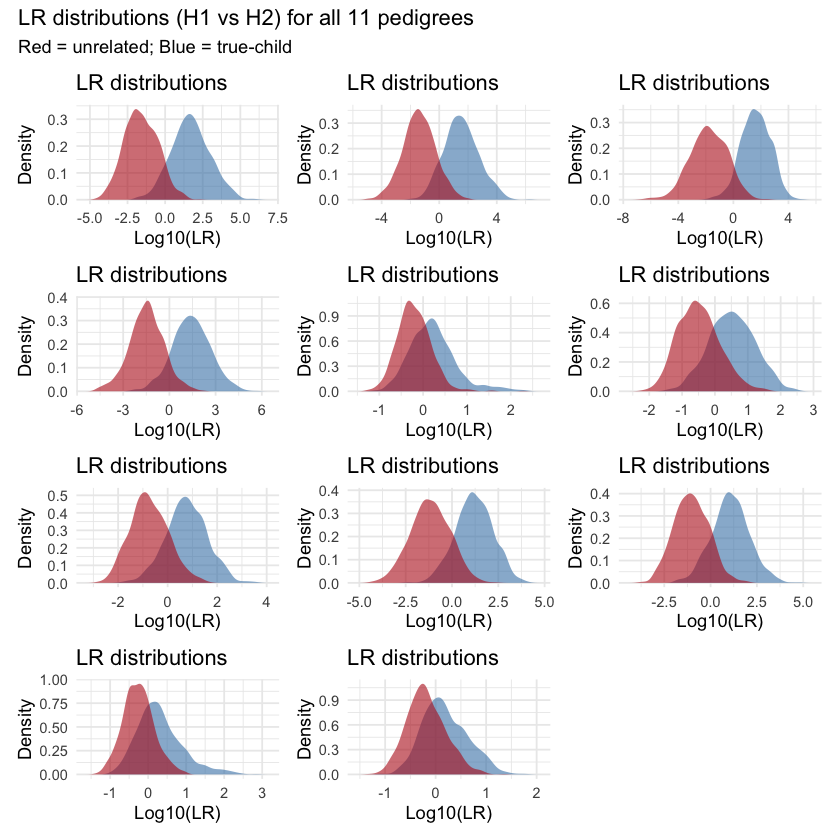
Table 2: LR plots.
For practical purposes, we would like to have a simple metric to measure how these curves overlap. To quantify how much the red and blue LR distributions overlap in each plot, we followed a five-step process. First, we extracted the total likelihood ratios from each of the 1,000 simulations under both hypotheses (H1 = true child, H2 = unrelated) and transformed them using log10. Second, we computed kernel density estimates for each log10-distribution. Third, we defined a shared x-axis grid spanning the region where both densities have support. Fourth, we interpolated both density curves onto this grid. Finally, we computed the overlap area by summing the pointwise minimums of the two densities across the grid and multiplying by the grid spacing. This gave us a single overlap value between 0 and 1 for each pedigree.
Recently, dense SNPs panels have allowed good coverage of the genome. This can be used to identify Identity by Descent segments and then define relationships between individuals. This approach proved to be useful in Forensic Investigative Genetic Genealogy efforts. Nevertheless, the main methods rely on pairwise comparisons. Our aim is to propose an alternative approach to compute probabilities based on a given pedigree with multiple sequenced individuals. Approximate Bayesian Computation (ABC) offers a promising alternative in complex kinship scenarios. ABC uses simulations to generate expected genetic patterns under different hypotheses. These simulated datasets are then compared to the observed data using summary statistics, allowing us to approximate the posterior probability of each hypothesis.
ABC is especially well-suited for our context because it can incorporate full pedigrees, multiple genotyped relatives, and population-level allele frequencies, while flexibly handling genotyping error and missing data. This makes it a strong candidate for improving identification in human rights cases where biological relatives may span several generations.
This package is now maintained by Suisei Nakagawa and Franco Marsico.