On-the-Fly Atomistic Calculator

This is an on-the-fly atomistic calculator based on Gaussian Process Regression (GPR), designed as an add-on calculator for the Atomic Simulation Environment (ASE). It employs a hybrid approach, combining:

1. Base calculator: A high-fidelity ab initio calculator (e.g., DFT) that serves as the reference ("gold standard") for accurate but computationally expensive calculations.
2. Surrogate GPR calculator: A computationally inexpensive model trained on-the-fly to approximate the base calculator, significantly accelerating simulations.

Motivation

Many atomistic simulations, such as geometry optimizations, barrier calculations (e.g., NEB), molecular dynamics (MD), and equation-of-state (EOS) simulations, require sampling a large number of atomic configurations within a relatively small phase space. Density Functional Theory (DFT) is frequently used for these calculations, offering a balance between accuracy and computational cost. However, DFT calculations can still be prohibitively expensive, especially for large systems or long simulation times. The GPR calculator aims to alleviate this computational bottleneck. At the moment, we focus on the NEB simulation only.

How It Works?

The GPR calculator operates through an iterative learning and prediction process:

1. Initial Data Collection: The simulation begins by using the base calculator (e.g., DFT) to calculate energies and forces for a small set of initial atomic configurations. These data serve as the initial training set for the GPR model.
2. Surrogate Model Training: A Gaussian Process Regression (GPR) model is trained using the data obtained from the base calculator. This model learns to predict the energy and forces of new atomic configurations based on the existing training data.
3. On-the-Fly Prediction and Uncertainty Quantification: During the simulation, for each new atomic configuration, the GPR model predicts the energy and forces, along with an estimate of the uncertainty in these predictions.
4. Choice of Calculator: The GPR calculator adaptively decides whether to use the GPR model's prediction or to invoke the base calculator based on the predicted uncertainty.
   • If the uncertainty is below a user-defined threshold, the GPR model's prediction is used, saving computational cost.
   • If the uncertainty is above the threshold, the base calculator is invoked to obtain a more accurate calculation. The new data point is then added to the training set, and the GPR model is retrained.
5. Iterative Refinement: Steps 3 and 4 are repeated throughout the simulation. As the GPR model accumulates more data, its accuracy improves, leading to a greater reliance on the surrogate model and a reduction in the number of calls to the base calculator.

This adaptive strategy allows the GPR calculator to achieve a balance between accuracy and computational efficiency, by using the computationally expensive base calculator only when necessary.

Installation

pip install .

A quick example

Below illustrates an example to run NEB calculation with the hybrid calculator

from ase.calculators.emt import EMT
from gpr_calc.gaussianprocess import GP
from gpr_calc.calculator import GPR
from gpr_calc.NEB import neb_calc, init_images, neb_plot_path

# Set parameters
init = 'examples/database/initial.traj'
final = 'examples/database/final.traj'
num_images = 5
fmax = 0.05

# Run NEB with EMT calculator
images = init_images(init, final, num_images)
images, engs, steps = neb_calc(images, EMT(), fmax=fmax)
data = [(images, engs, f'EMT ({steps*(len(images)-2)+2})')]

# Run NEB with gpr calculators
for etol in [0.02, 0.1, 0.2]:
    images = init_images(init, final, num_images)

    # initialize GPR model
    gp_model = GP.set_GPR(images, EMT(),
                          noise_e=etol/len(images[0]),
                          noise_f=0.1)
    # Set GPR calculator
    calc = GPR(base=EMT(), ff=gp_model, save=False)

    # Run NEB calculation
    images, engs, _ = neb_calc(images, calc, fmax=fmax)
    N_calls = gp_model.count_use_base
    data.append((images, engs, f'GPR-{etol:.2f} ({N_calls})'))
    print(gp_model, '\n\n')

neb_plot_path(data, figname='NEB-test.png')

This example demonstrates NEB calculations using:

1. A pure EMT calculator (for rapid testing).
2. A GPR calculator with EMT as the base and an uncertainty threshold of 0.02 eV per structure.
3. A GPR calculator with EMT as the base and an uncertainty threshold of 0.10 eV per structure.
4. A GPR calculator with EMT as the base and an uncertainty threshold of 0.20 eV per structure.

The output below illustrates the NEB calculation process. Initially, the base calculator (EMT) is used to generate reference data. These data points are then added to the GPR model. As the model learns and becomes more accurate, predictions from the surrogate model are used more frequently, reducing the computational cost.

Calculate E/F for image 0: 3.314754
Calculate E/F for image 1: 3.727147
Calculate E/F for image 2: 4.219952
Calculate E/F for image 3: 3.724974
Calculate E/F for image 4: 3.316117
------Gaussian Process Regression (0/2)------
Kernel: 1.00000**2 *RBF(length=0.10000) 5 energy (0.00769) 15 forces (0.10000)

Update GP model => 20
Loss:       -2.916  1.000  0.100
Loss:     1821.480  0.010 10.000
Loss:       48.811  0.527  4.827
Loss:      -51.328  0.835  1.750
Loss:      -52.140  0.898  1.717
Loss:      -53.035  1.025  1.634
Loss:      -53.163  1.078  1.589
From Surrogate ,  E: 0.054/0.100/3.729, F: 0.102/0.120/1.660
From Surrogate ,  E: 0.066/0.100/4.215, F: 0.155/0.120/3.489
From Surrogate ,  E: 0.054/0.100/3.725, F: 0.102/0.120/1.651
      Step     Time          Energy          fmax
BFGS:    0 20:02:22        4.214882        3.489110
From Surrogate ,  E: 0.054/0.100/3.647, F: 0.103/0.120/1.284
From Surrogate ,  E: 0.066/0.100/3.918, F: 0.154/0.120/2.609
From Surrogate ,  E: 0.053/0.100/3.644, F: 0.103/0.120/1.278
BFGS:    1 20:02:24        3.917948        2.608887
From Base model , E: 0.053/3.500/3.546, F: 0.182/0.350/0.400
From Base model , E: 0.100/3.512/3.738, F: 0.315/0.423/0.434
From Base model , E: 0.053/3.499/3.545, F: 0.183/0.349/0.399
BFGS:    2 20:02:29        3.737970        0.488517
...
...
...
From Surrogate ,  E: 0.095/0.200/3.694, F: 0.062/0.120/0.039
From Surrogate ,  E: 0.081/0.200/3.526, F: 0.097/0.120/0.391
BFGS:   41 20:08:35        3.693717        0.039118
From Surrogate ,  E: 0.082/0.200/3.344, F: 0.069/0.120/0.041
From Surrogate ,  E: 0.082/0.200/3.346, F: 0.067/0.120/0.048
------Gaussian Process Regression (0/2)------
Kernel: 2.80314**2 *RBF(length=1.52921) 7 energy (0.01538) 55 forces (0.10000)
Total base/surrogate/gpt_fit calls: 22/106/4

The trained GPR model is saved as:

• A json file containing the model parameters.
• A db file storing the training structures, energies, and forces.

The following figure illustrates a typical NEB path calculated using the GPR calculator:

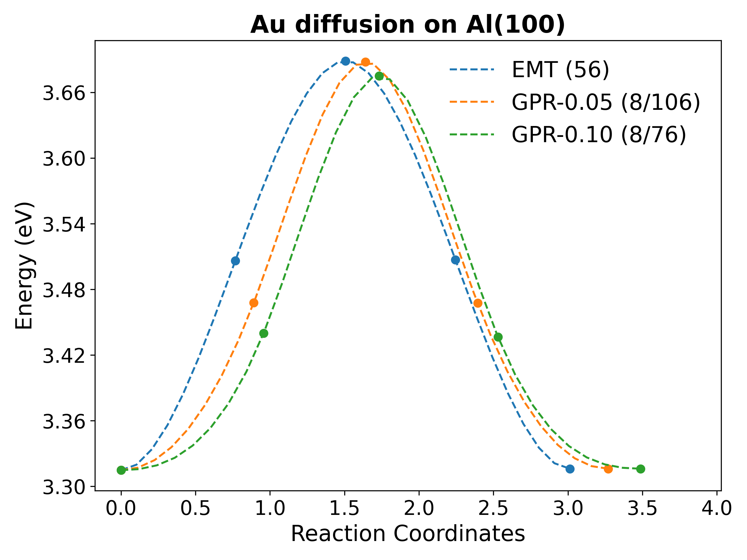
The results demonstrate that the GPR calculator, even with a limited number of base calculator calls, can achieve reasonable accuracy compared to the reference calculation. A smaller energy uncertainty threshold (etol) generally leads to more accurate results. In scenarios where each base calculator call is computationally expensive, the GPR calculator offers a significant speedup without sacrificing accuracy. This approach is particularly beneficial for handling computationally demanding tasks such as large-scale NEB calculations for surface diffusion and reaction studies.

In addition, the trained model can be reused as follows if you want to restart the previously unconverged calculation.

from gpr_calc.gaussianprocess import GPR

gpr = GPR.load('test-RBF-gpr.json')
print(gpr)
gpr.validate_data(show=True)
gpr.fit(opt)

For more productive examples using VASP as the base calculator, please check the Examples.