Dual-Architecture Machine Learning System Using LightGBM & Temporal Convolutional Networks for Early Warning in Critical Care
Dual-architecture machine learning system for early detection of clinical deterioration in intensive care unit (ICU) patients. The system compares gradient-boosted decision trees (LightGBM) with temporal convolutional networks (TCN) to model complementary aspects of physiological risk using routinely collected clinical observations. Three NEWS2-derived deterioration outcomes are considered: maximum risk level attained during the ICU stay (max_risk), median sustained risk level across the stay (median_risk), and the proportion of time spent in a high-risk state (pct_time_high).
Models are trained and evaluated using the PhysioNet MIMIC-IV Clinical Demo v2.2 dataset via two distinct feature-engineering pipelines. The TCN operates on high-resolution timestamp-level temporal features (96-hour windows, 171 features) to capture short-term physiological instability, while the LightGBM model uses patient-level aggregated tabular features (40 features) to characterise longer-term exposure to risk. Comparative evaluation indicates complementary performance profiles: LightGBM exhibits superior calibration and regression fidelity for sustained risk estimation, while TCNs show stronger sensitivity and discrimination for acute deterioration events. Performance is assessed using ROC-AUC, Brier score, and R², alongside interpretability analyses based on SHAP values and saliency methods.
The end-to-end pipeline includes clinically validated NEWS2 preprocessing of 70,640 time-stamped measurements over 140 ICU stays (including CO₂ retainer logic, Glasgow Coma Scale mapping, and supplemental oxygen protocols), comprehensive feature engineering, model training with hyperparameter optimisation, robust metric evaluation, and a command-line inference interface supporting batch prediction and per-patient lookup. Overall, the system demonstrates physiologically plausible predictive behaviour, clinically meaningful interpretability, and a reproducible workflow suitable for extension to full clinical datasets or downstream deployment contexts.
The use of a limited demo dataset (100 patients across 140 ICU stays) constrains statistical reliability and generalisability. As a result, reported performance metrics (e.g., ROC-AUC, R²) are likely optimistic and should not be interpreted as clinically valid estimates of real-world performance. The primary objective of this work is to demonstrate pipeline design, feature engineering, and comparative model behaviour under constrained data conditions, rather than to establish definitive predictive accuracy. In a production or research setting, this framework would be extended to the full MIMIC-IV dataset with appropriate patient-level splits, cross-validation, and uncertainty estimation to support robust evaluation.
This repository contains code, preprocessed outputs, and documentation only; no raw clinical data is redistributed. Users must obtain the MIMIC-IV dataset directly from PhysioNet and comply with its data use requirements. The work is intended for research and educational use.
| Target Outcome | Best-Performing Model | Key Metric(s) | Notes |
|---|---|---|---|
max_risk |
TCN | ROC-AUC = 0.923 | Strong acute deterioration detection |
median_risk |
LightGBM | ROC-AUC = 0.972; Brier Score = 0.065 | Superior sustained risk calibration |
pct_time_high |
LightGBM | R² = 0.793; RMSE = 0.038 | Higher fidelity estimation of high-risk exposure |

Figure: Temporal CCN (TCN) architecture used for timestamp-level prediction
Technical stack: Python, PyTorch, Scikit-learn, LightGBM, pandas, NumPy
Expand table of contents
- Clinical Background & Motivation
- Project Goals & Contributions
- Phase 1 - Data Extraction & NEWS2 Computation
- Phase 2 - Feature Engineering (Timestamp & Patient-Level)
- ML Modelling Strategy
- Phase 3 — LightGBM Pipeline: Baseline Modelling & Hyperparameter Tuning
- Phase 4 — Temporal Convolutional Network (TCN) Pipeline: Architecture & Training
- Phase 5 – Evaluation: Metrics & Interpretation
- Phase 6A – Comparative Analysis: LightGBM vs TCN
- Phase 6B – Interpretability: LightGBM SHAP vs TCN Saliency
- 10.1 Why Interpretability Matters in Clinical ML
- 10.2 How Interpretability Fits Into Phase 6
- 10.3 LightGBM Interpretability: SHAP Background & Overview
- 10.4 LightGBM Interpretability: SHAP Results & Interpretation
- 10.5 TCN Interpretability: Saliency Overview & Rationale
- 10.6 TCN Interpretability: Saliency Results & Interpretation
- 10.7 SHAP vs Saliency: Cross-Model Interpretability
- Phase 7 – Inference Demonstration (Deployment-Lite)
- Methodological Rationale and Design Reflection
- Limitations
- Future Work
- Potential Clinical Integration
- Repository Structure
- How to Run
- Requirements & Dependencies
- License
- Copyright
- Citation
- Acknowledgments
ICU patient deterioration often emerges through subtle physiological changes hours before critical events. The National Early Warning Score 2 (NEWS2) is widely used in UK hospitals to detect and escalate care for deteriorating patients. Accurate, real-time scoring and risk stratification can:
- Enable earlier intervention and ICU escalation
- Support clinical decision-making with actionable, interpretable metrics
- Provide a foundation for advanced ML-based early warning systems
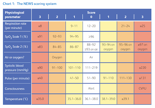
Figure: INTEROPen NHS Digital. NEWS2 Implementation Guide
Although the national standard for deterioration detection, NEWS2 has well-recognised constraints:
- No temporal modelling: Although observations are charted sequentially, the scoring algorithm treats each set of vitals independently and does not incorporate trend, slope, variability, or rate-of-change.
- Discrete scoring limitations: continuous physiological signals are combined into discrete scores and does not model interactions between multiple variables, limiting sensitivity to subtle multivariate deterioration patterns.
- Escalation overload: Threshold-based triggers produce high false-positive rates in elderly and multimorbid cohorts, contributing to alert burden and escalation fatigue.
- Limited predictive horizon: Escalation only occurs after thresholds are breached, restricting early-warning capability.
NEWS2 scoring bands map directly to clinical monitoring frequency and escalation actions; these operational consequences define the clinical targets we aim to predict:
| NEWS2 Score | Clinical Risk | Monitoring Frequency | Clinical Response |
|---|---|---|---|
| 0 | Low | Minimum every 12h | Routine monitoring by registered nurse. |
| 1–4 | Low | Minimum every 4-6h | Nurse to assess need for change in monitoring or escalation. |
| Score of 3 in any parameter | Low–Medium | Minimum every 1h | Urgent review by ward-based doctor to decide monitoring/escalation. |
| 5–6 | Medium | Minimum every 1h | Urgent review by ward-based doctor or acute team nurse; consider critical care team review. |
| ≥7 | High | Continuous monitoring | Emergent assessment by clinical/critical-care team; usually transfer to HDU/ICU. |
- Transitions between these risk categories directly influence clinical workload and resource allocation, including urgent reviews and ICU involvement.
- Predicting imminent transitions into these categories (e.g., entering high risk within the next 4–6 hours) enables earlier intervention, reducing delayed escalations and improving critical-care resource planning.
- NEWS2 is the national standard for ward-based clinical deterioration assessment and provides a clinically validated ground-truth for model training and evaluation.
- The ML models predict summary outcomes derived from NEWS2 clinical-risk categories:
max_risk: Maximum risk attained during staymedian_risk: Average sustained risk across the staypct_time_high: Percentage of time spent in high-risk state
- Evaluating ML predictions against these NEWS2-derived outcomes allows assessment of predictive horizon, sensitivity, and the ability to anticipate clinically actionable deterioration trends before standard escalation would occur.
ICU deterioration involves complex and often subtle, multivariate temporal patterns that standard threshold-based systems cannot fully capture. Machine learning enables prediction of clinically meaningful NEWS2-derived outcomes using both static and temporal representations of patient physiology.
| Model | Type | Input Features | Modelling Type | Strengths | Weaknesses | Interpretability |
|---|---|---|---|---|---|---|
| LightGBM | Gradient-Boosted Decision Tree (GBDT) | Aggregated patient-level | Static | Fast, interpretable, good calibration | Cannot capture sequential dynamics | SHAP |
| TCN | Temporal Convolutional Network | Timestamp-level sequential | Temporal | Captures temporal trends, slopes, variability | More computationally intensive than tree-based, less interpretable, requires careful hyperparameter tuning | Saliency (grad×input) |
- Strong baseline for structured, tabular data like patient-level aggregations of vitals and summary statistics.
- Captures non-linear interactions between vital signs
- Fast to train and tune, handles missing values natively
- Highly interpretable via SHAP, critical for clinician understanding
- Often competitive or superior when temporal structure is weak
- Models long-range temporal context and time-dependent patterns
- Robust to irregular sampling frequency (measurement intervals)
- Learns patterns in timestamp-level features, detecting short-term deterioration trends and acute changes that static models may miss.
- LightGBM evaluates performance on static, aggregated patient-level data.
- TCN uses temporal modelling to capture complex, sequential patterns from timestamp-level data.
- Comparison reflects realistic deployment: classical ML may suffice for long-term sustained deterioration patterns, whereas temporal models exploit high-resolution monitoring to detect early deterioration.
- This identifies where temporal modelling adds value, where classical ML suffices, and the trade-offs between performance and interpretability.
This project therefore systematically evaluates temporal vs. non-temporal ML approaches for predicting ICU deterioration using clinically meaningful NEWS2-derived targets.
- Establish a clinically validated deterioration-prediction framework by using NEWS2-derived risk categories as the reference standard for all model targets and evaluation.
- Compare classical vs. deep learning to quantify the added predictive value of temporal modelling by systematically comparing a static gradient-boosted decision tree model (LightGBM) against a temporal convolutional network (TCN) on the same patients and targets.
- Design dual feature engineering pipelines (timestamp-level for TCN, patient-level for LightGBM) incorporating temporal statistics, imputation, and missingness flags; aligned with real hospital data quality constraints.
- Evaluate model performance across 3 risk horizons to ensure fair model comparison, demonstrating how different architectures capture acute vs. long-term physiological instability.
- Implement transparent model-specific interpretability pathways (SHAP vs. saliency) to ensure outputs remain clinically aligned and defensible, supporting clinician trust during decision-making and escalation.
- Develop an end-to-end, deployment-lite inference system capable of running batch and per-patient predictions, enabling direct applicability to real-world ICU or ward settings.
- Dual-Model Feature Engineering: Built a reproducible pipeline from raw EHR data, including feature extraction, NEWS2 computation (GCS→LOC mapping, CO₂ retainer and supplemental O₂ rules), and clinically interpretable timestamp- and patient-level features (LOCF, missingness flags, rolling windows, summary statistics).
- LightGBM Baselines: Developed robust patient-level models with binary target handling for sparse classes, stratified cross-validation, and hyperparameter tuning for stable, reproducible performance.
- TCN Architecture: Designed multi-task temporal convolutional network for time-series data, combining causal dilated convolutions, residual connections, and masked mean pooling.
- Evaluation & Diagnostics: Built unified evaluation utility for reproducible metrics; diagnosed and corrected TCN metric misalignment to restore true ROC-AUC.
- Model Retraining & Stability: Implemented targeted TCN retraining with class-weighted BCE and log-transform regression, preserving architecture and hyperparameters while improving convergence and predictive reliability.
- Comprehensive Analysis Pipeline: Executed unbiased test set inference, TCN calibration/threshold tuning, and cross-model comparative analysis for LightGBM vs. TCN.
- Interpretability & Deployment: Delivered global SHAP feature explanations (LightGBM) and gradient×input saliency maps (TCN), and packaged a unified, lightweight inference pipeline supporting batch and interactive per-patient predictions with deterministic, dataset-agnostic outputs.
- Overview: Medical Information Mart for Intensive Care (MIMIC)-IV database is comprised of deidentified patient electronic health records, taken from PhysioNet.org.
- Contents: 26 tables of structured vital signs, labs, and admission data; excludes free-text clinical notes.
- Patients: 100 ICU admissions (de-identified subset)
- Tables used:
chartevents,patients,admissions,d_items - Limitations: Small sample size (full dataset contains >65,000 ICU admissions), limited high-risk events.
Goal: Extract relevant vital signs, encode clinical rules, compute NEWS2 scores per timestamp and per patient producing reproducible outputs for feature engineering.
                          Raw MIMIC-IV CSVs
                    (chartevents, patients, etc.)
                                  │
                        extract_news2_vitals.py
                                  │
                                  ▼
          news2_vitals_with_co2.csv + co2_retainer_details.csv
                                  │
                          compute_news2.py
                                  │
                  ┌───────────────┴───────────────┐
                  ▼                               ▼
  news2_scores.csv (timestamp-level)   news2_patient_summary.csv (patient-level)
The pipeline extracts all NEWS2-relevant physiological variables using universal encoding labels, including custom CO2 retainer logic implementation. NEWS2 parameter scoring and total scoring is implemented, with both timestamp-level and patient-level files being created.
| Parameter | Range | NEWS2 Points |
|---|---|---|
| Respiratory Rate | ≤8 → ≥25 | 0–3 |
| SpO₂ (Scale 1) | ≤91 → ≥96 | 0–3 |
| SpO₂ (Scale 2, hypercapnic) | ≤83 → ≥97 | 0–3 |
| Supplemental O₂ | No / Yes | 0 / 2 |
| Temperature | ≤35°C → ≥39.1°C | 0–3 |
| Systolic BP | ≤90 → ≥220 | 0–3 |
| Heart Rate | ≤40 → ≥131 | 0–3 |
| Level of Consciousness | Alert / Not Alert | 0 / 3 |
(Discrete NHS NEWS2 bands are applied in code; the table above shows compressed min–max ranges.)
- CO₂ Retainer Identification
All ABG measurements in `chartevents.csv` examined. Criteria (all must be met):
- PaCO₂ > 45 mmHg (chronic hypercapnia)
- pH 7.35-7.45 (compensated respiratory acidosis)
- ABG measurements ±1 hour apart
→ Triggers SpO₂ Scale 2 (target 88-92% vs 94-98%). No patients in current dataset met criteria.
- GCS → Level of Consciousness (LOC) Mapping
Combine column scores (`GCS - Eye Opening`, `GCS - Verbal Response`, `GCS - Motor Response`) to create `gcs_total`.
- GCS ≥15: Alert (LOC = 0)
- GCS <15: Not Alert (LOC = 3)
→ Non-alert states add +3 to NEWS2
- Supplemental O₂ Detection
FiO₂ can be identified via `Inspired O2 Fraction` in CSV and converted to binary supplemental O₂ indicator.
- ≤0.21 = not on supplemental O₂ (0)
- >0.21 = on supplemental O₂ (1)
→ Any supplemental O₂ adds +2 to NEWS2
Timestamp-level: news2_scores.csv
- One row per observation timestamp
- Raw vitals, individual parameter scores, total NEWS2 score
- Supplemental O₂, CO₂ retainer, and consciousness/GCS labels.
- Escalation risk category (low/medium/high), monitoring frequency, response.
Patient-level: news2_patient_summary.csv
- Per-patient aggregations: min, max, mean, median, total number of timestamps
- Summary statistics per patient.
Purpose: Transform NEWS2 data into patient-level + timestamp-level ML-ready feature-sets for tree-based models (LightGBM) and Neural Networks (TCN).
                              news2_scores.csv
                                       │
             ┌─────────────────────────┴─────────────────────────┐
             │                                                   │
  make_patient_features.py                           make_timestamp_features.py
             │                                                   │
             ▼                                                   ▼
  Patient-Level Feature Engineering                  Timestamp-Level Feature Engineering
  - Median, mean, min, max per vital                 - Missingness flags
  - Imputation using patient-specific median         - Last Observation Carried Forward (LOCF)
  - % Missingness per vital                          - Carried-forward flags
  - Encode risk labels and summary target stats      - Rolling windows 1/4/24h (mean, min, max, std, slope, AUC)
      • max_risk                                     - Time since last observation (staleness)
      • median_risk                                  - Encode risk labels
      • pct_time_high                                            │
             │                                                   │
             ▼                                                   ▼
  news2_features_patient.csv                        news2_features_timestamp.csv
             │                                                   │
             ▼                                                   ▼
  LightGBM Model (Classical ML)                     Temporal Convolutional Network (TCN)
- Timestamp-level features: Provide the richest representation, capturing short-, medium-, and long-term deterioration patterns. Essential for sequence-based models like deep learning architectures (e.g., TCN).
- Patient-level features: Aggregated summaries of vital signs, useful for testing simpler models, evaluating feature importance, and establishing baseline metrics.
Maintaining both feature sets ensures flexibility and robustness in model selection:
- LightGBM → clinician-friendly, interpretable baseline using patient-level features.
- TCN → modern deep learning approach leveraging full temporal sequences to capture dynamic deterioration trends.
Purpose: Capture temporal dynamics for sequential modeling
Imputation Strategy
- Missingness flags: Binary indicators (1/0) for each vital parameter (value carried forward=1) so models can learn from missing patterns. Before carried-forward so that it is known which values were originally missing.
- LOCF (Last Observation Carried Forward) flags: Propagate previous valid measurement, and create a binary carried-forward flag (binary 1/0).
Rolling Window Features (1/4/24h)
- Mean: Average value
- Min/Max: Range boundaries
- Std: Variability
- Slope: Linear trend coefficient
- AUC (Area Under Curve): Integral of value over time
Other Features
- Staleness: Time since last observation (staleness per vital)
- Numeric risk encoding: Encoded as 0 (low), 1 (medium-low), 2 (medium), 3 (high)
- Timestamp-level:
news2_features_timestamp.csv - ML-ready per patient per timestamp features (ordered by
subject_idand bycharttime). - Full time-series per patient allows modelling of temporal patterns, trends, dynamics
(total_timestamps, n_features) = (20,814 timestamps, 136 features)
- 136 features =
- Rolling windows → 5 vitals x 3 windows x 6 stats = 90
- 8 vitals x (staleness + missingness flag + LOCF flag) = 24
- 14 raw clinical signals + 3 derived clinical labels = 17
- NEWS2 → NEWS2 score + risk label + monitoring frequency + response + numeric risk = 5
Purpose: Aggregated risk profile for interpretable tree-based modeling
- Vital sign aggregations (per parameter): Median, mean, min, max
- Patient-specific median imputation: Fill missing values for each vital (preserves patient-specific patterns), if a patient never had a vital recorded, fall back to population median.
- % Missingness per vital: track proportion of missing values pre-imputation, data quality indicator, signal from incomplete measurement pattern.
- Escalation summary metrics: convert risk label to numeric then compute
max_risk= maximum risk attainedmedian_risk= average sustained riskpct_time_high= % time spent in high-risk state
- Patient-level:
news2_features_patient.csv - ML-ready per patient aggregated summary features (ordered by
subject_id) - One row per patient (fixed-length vector).
(n_patients, n_features) = (100, 43)
- 43 features =
- 8 vitals x (median + mean + min + max + % missing) = 40
- Summary features →
max_risk+median_risk+pct_time_high= 3
| Model | Input Resolution | Architecture Type | Mechanism | Primary Strength | Clinical Application |
|---|---|---|---|---|---|
| LightGBM | Patient-aggregated (40 features) | Gradient-boosted decision trees | Builds an ensemble of decision trees sequentially using gradient-based optimization; each tree corrects residual errors of previous trees to minimize loss | Calibrated probability estimates, strong interpretability, robust baseline | Sustained risk stratification, resource allocation, triage scoring |
| TCN | Timestamp-sequential (96×171 tensor) | Temporal convolutional network | Applies causal, dilated convolutions with residual connections over sequential inputs to capture long-range temporal dependencies efficiently | Temporal pattern detection, high acute-event sensitivity | Real-time monitoring, rapid deterioration alerts, dynamic forecasting |
- LightGBM (Classical ML): Establishes transparent, clinician-interpretable baseline and identifies which vitals matter most at the patient-level.
- TCN (Deep Learning): Advances to time-series modeling which captures temporal dependencies, demonstrating how deterioration unfolds dynamically over time, which captures dynamics that aggregated features can’t.
- Combining the two showcases progression from classical tabular ML → modern sequence-level deep learning, proving competence across both paradigms.
- Acute detection: Requires high-sensitivity to short-term trend changes (TCN advantage)
- Sustained risk: Requires calibrated probability estimates over full stay (LightGBM advantage)
- Dual architecture approach represents two distinct clinical tasks; sustained risk assessment + acute monitoring, pipeline leverages each model's inherent strengths by aligning to its optimal prediction task.
| Model | Strengths | Limitations | Decision Rationale |
|---|---|---|---|
| Logistic Regression (Linear) | Simple, fast, easy to deploy, interpretable coefficients | Linear assumptions; cannot model non-linear vital-sign interactions, tends to underperform on raw time-series vitals | Insufficient for complex ICU physiological patterns |
| Random Forest (Bagged Trees) | Robust, ensemble tree-based method; handles nonlinearities; less sensitive to scaling | Slower and less sample-efficient than boosted trees; weaker performance on small datasets | Boosted trees outperform on structured EHR data |
| XGBoost (Boosted Trees) | Industry-standard GBDT; good regularisation; mature ecosystem | Slower training, higher memory usage | Comparable, but suboptimal for small 100-patient dataset |
| CatBoost (Boosted Trees) | Excellent handling of categorical features; stable training | Benefits irrelevant when features are already numeric | No categorical variables → added complexity gives no gain |
| LightGBM (Boosted Trees) | Fastest GBDT, highly efficient, handles NaNs natively, efficient SHAP integration | Requires careful hyperparameter tuning to avoid overfitting on small samples | Best choice for small tabular datasets with missingness |
- Most efficient GBDT for small tabular datasets → faster and lighter than XGBoost/CatBoost, ideal for a 100-patient regime.
- Native missing-value handling (NaNs) → tree-splitting logic automatically routes missing values, avoiding imputation pipelines (beyond simple patient-median fallback).
- Rapid training/evaluation → enables fast experimentation and iteration across multiple targets and CV folds.
- Efficient SHAP integration for interpretability → SHAP values directly explain tree splits, giving exact feature attribution, critical for clinical transparency.
- Proven performance → boosted trees consistently outperform linear models and shallow learners on structured EHR/ICU tabular data
| Standard / Core | Strengths | Limitations | Decision Rationale |
|---|---|---|---|
| LSTM/GRU (Recurrent) | Well-suited for sequences, handles variable-length inputs | Vanishing gradients on long sequences, slow sequential training | Unstable gradients on long ICU sequences, computationally inefficient, dataset too small for deep RNN stacks |
| Transformer (Self-attention) | Powerful for long sequences, models global dependencies | Requires large datasets for self-attention to learn effectively, computationally intensive, prone to overfitting | Overkill for small dataset; unnecessary complexity |
| TCN (Convolutional) | Parallelizable, dilated convolutions, stable gradients, captures long-range temporal dependencies | Requires sequence padding, normalisation, masking for missingness | Efficient and robust for small-sample ICU time-series; best balance of performance and practicality |
| Specialised / Niche | Strengths | Limitations | Decision Rationale |
|---|---|---|---|
| Neural ODE (continuous-time) | Continuous-time dynamics instead of discrete layers | Niche research technique, slow, unstable complex training (ODE solvers) | Rarely production-ready, not clinically validated |
| Graph Neural Network (GNN) | Models patient-patient similarity or hospital network relationships | Requires graph structure, not sequences or grids; operates on node/edges | Inapplicable to independent patient time-series |
| WaveNet (Autoregressive) | Deep, heavy convolutional autoregressive model for audio | Designed for massive datasets (speech), computationally huge | Impractical and slow for 100-patient clinical dataset |
- Modern, credible sequence architecture → advanced enough to demonstrate deep-learning capability without appearing niche or experimental.
- Dilated causal convolutions → capture long physiological context windows while preventing future leakage.
- Fully parallel convolutional operations → train faster and more efficiently than sequential RNNs.
- Residual connections stabilise gradients → avoid vanishing/exploding issues common in RNNs (LSTMs/GRUs).
- Fewer parameters than Transformers → suitable for small clinical datasets without overfitting risk.
- Inductive bias for local temporal patterns → aligns with how ICU deterioration emerges through short-term trends and slopes.
- Exponential receptive field → models long ICU stays without needing deep recurrent stacks.
- Temporal saliency maps → reveal when features influenced predictions, enabling time-aware interpretability.
- Strong empirical support → consistently outperforms RNNs on moderate-length clinical sequences; well-validated in medical ML literature (unlike Neural ODEs, GNNs, WaveNet).
Temporal awareness:
- Causal convolutions → at each time step, the model only looks backwards in time (no data leakage from the future).
- Dilated convolutions → skip connections expand the receptive field exponentially, captures long-range temporal patterns without deep stacking (without needing hundreds of layers).
Stable training:
- Residual blocks → stabilise gradient flow, prevent vanishing/exploding gradients, making the deep temporal model easier to optimise.
From sequences to predictions:
- Global pooling → compresses full sequence into a single fixed-length representation.
Rationale: Patient-level outcomes ensure that the TCN’s predictions are directly comparable with LightGBM while still taking advantage of temporal trends in ICU sequences.
TCN Approach
- Input / Features: Timestamp-level sequences → captures full temporal patterns.
- Targets: Patient-level outcomes (
max_risk,median_risk,pct_time_high). - Training approach: Each timestep inherits the patient label → TCN maps whole sequence → patient-level prediction.
Why not per-timestep prediction
- True sequence-to-sequence labeling would predict risk per timestep for richer early-warning capability.
- Challenges: require detailed labels for every timestamp (rare in ICU datasets), per-timestep prediction in a small dataset is prone to overfitting and instability; and evaluation is complex.
| Aspect | LightGBM (Classical ML) | Current TCN | Full TCN Potential |
|---|---|---|---|
| Input format | Patient-level aggregates news2_features_patient.csv |
Timestamp-level sequences (padded) news2_features_patient.csv |
Timestamp-level sequences (padded) news2_features_patient.csv |
| Targets | max_risk, median_risk, pct_time_high |
max_risk, median_risk, pct_time_high |
Per-timestep risk (hourly escalation) |
| Features | Aggregated stats (mean, median, min, max, % missing) | Rolling windows + LOCF + missingness + staleness | Same + explicit per-timestep features |
| Temporal modeling | None (static aggregates) | Captures temporal trends across full sequences | Captures full temporal patterns and enables per-timestep early-warning predictions |
| Interpretability | SHAP (feature-level) | Saliency maps over features & time (sequence-level) | Saliency + per-timestep attributions (fine-grained temporal insight) |
| Computational complexity | Low | Moderate | High |
| Strengths | Robust, credible baseline | Detects deterioration trajectories | Detects trajectories + predicts escalation |
| Portfolio value | Demonstrates baseline competency | Shows advanced temporal modeling | Demonstrates sequence-level ML mastery |
Why patient-level labels are appropriate:
- Clinical relevance: Clinicians care whether escalation occurred, not exactly when.
- Data constraints: Sparse or missing per-timestep labels make sequence-to-sequence modeling unreliable.
- Comparison clarity: Aligns TCN outcomes with LightGBM for direct performance comparison.
- Portfolio value: Demonstrates temporal modeling capability without unnecessary complexity.
- Practicality: Reduces coding/debugging overhead while preserving temporal advantage.
Key insight:
- Patient-level TCN outputs leverage temporal patterns that LightGBM cannot capture.
- Sequence-to-sequence prediction is technically feasible but impractical here; this approach balances complexity with feasbility and dataset constraints.
| Dimension | LightGBM (GBDT) | TCN (Temporal CNN) |
|---|---|---|
| Data Requirement | Works well on small tabular datasets (≤100 patients) | Requires timestamp-level sequences; benefits from richer data |
| Temporal Awareness | None — uses aggregated features | Strong — captures short- and long-range trends via dilated convs |
| Training Efficiency | Extremely fast, low compute | Moderate — parallel but more computationally heavy |
| Overfitting Risk | Low with tuned parameters | Higher if sequences are long or dataset small |
| Interpretability | Excellent (SHAP, tree splits) | Moderate (saliency maps) |
| Clinical Strength | Calibrated sustained-risk estimation | Acute deterioration detection in real time |
| When It Excels | Low-frequency data, small datasets, need for transparency | High-frequency temporal data, subtle deterioration patterns |
| When It Struggles | Fails to capture time-dependent dynamics | Requires more preprocessing (padding, normalisation, masking) and careful architecture tuning (kernel size, dilation, layers) |
Purpose: Establish classical ML baseline, identify dataset properties, and produce stable hyperparameters for downstream evaluation.
                                      news2_features_patient.csv
                                                  │
              ┌──────────────────────────┬────────┴───────────────┬───────────────────────┐
  complete_train_lightgbm.py    feature_importance.py   train_final_models.py       tune_models.py
              │                          │                        │                       │
              ▼                          ▼                        ▼                       ▼
  Preprocessing + CV Training   Feature Importance      Final Models               Hyperparameter Tuning
  (baseline models)             (per-fold)              (3 deployed LGBMs)         (only retained output)
  - Class collapse +            - Aggregated across     - Full-dataset models      - 5-fold CV grid search
  binarisation                  folds                   - Deployment-ready .pkls   - Tuning run logs per target
  - 5-fold CV (15 models)       - Bar plots + CSVs                │                - best_params.json
  - Fold metrics                       │                          │                       │
              │                        │                          │                       │
              ▼                        ▼                          ▼                       ▼
    Superseded by Phase 5     Superseded by Phase 6     Superseded by Phase 5    Retained for Phase 5
    (evaluation pipeline)     (SHAP interpretability)   (retraining)             (retraining and evaluation)
- Class handling: Identified severe class imbalance and rare-events carcity → applied target binarisation and stratified 5-fold CV to stabilise evaluation.
- Baseline modelling: Trained initial LightGBM classifiers/regressors on patient-level features (5-fold CV → 15 baseline models + metrics).
- Hyperparameter tuning: Per-target tuning of
learning_rate,max_depth,n_estimators,min_data_in_leaf→ producedbest_params.jsonused in later phases. - Feature importance: Generated fold-averaged LightGBM feature importance to confirm model signal (later superseded by Phase 6 SHAP).
- Final models: Trained full-cohort deployment-style final models using tuned hyperparameters (later superseded by Phase 5 retraining).
- A 5-fold CV LightGBM baseline was run to validate pipeline correctness, expose dataset issues, and establish a minimal working baseline before tuning.
- Models were trained on
news2_features_patient.csvfor 3 targets:- Classification:
max_risk+median_risk→ 5-fold StratifiedKFold - Regression:
pct_time_high→ 5-fold KFold
- Classification:
- Baseline runs revealed major dataset properties:
- Strong class imbalance and rare-event sparsity in both classification targets
max_risk+median_risk. - Clinically expected: severe deterioration (
max_risk=3) and sustained high-risk burden are uncommon.
- Strong class imbalance and rare-event sparsity in both classification targets
- Required class consolidation + binarisation:
- Binarisation improves model stability, simplifies clinical interpretation, and aligns with binary alert systems.
- Required StratifiedKFold:
- Essential to ensure each fold contained minority-class examples, avoid folds with absent classes, and reduce evaluation variance; critical with only 100 patients.
- Identifying these issues early ensured consistent binarisation and stratified sampling throughout later phases, making subsequent pipelines robust and reproducible on small, imbalanced clinical datasets.
| Target | Original Classes | Consolidated Classes | Binary Encoding Used in Training |
|---|---|---|---|
| max_risk | 0, 1, 2, 3 | 0/1/2 → 2 (not high risk), 3 → 3 (high risk) | 2 → 0, 3 → 1 |
| median_risk | 0, 1, 2, 3 | 0+1 → 1 (low), 2 → 2 (medium), 3 removed (no high risk in data) | 1 → 0, 2 → 1 |
- This is the only Phase 3 component used in later phases (Phase 5 LightGBM evaluation).
- Tuned the four parameters with the highest impact on stability and generalisation for small tabular datasets:
learning_rate→ controls step size; balances speed vs overfitting.max_depth/num_leaves→ limits tree complexity; prevents overfitting small dataset.n_estimators→ total number of trees.min_data_in_leaf→ ensures each leaf has enough samples,
- 5-fold CV evaluation:
- Classification (
max_risk,median_risk) → AUROC / Accuracy - Regression (
pct_time_high) → RMSE
- Classification (
- Why tuning was essential:
- Only 100 patients → high overfitting risk.
- These parameters dominate LightGBM performance on small data.
- Ensures LightGBM is fairly compared against TCN models in later phases.
- Generates stable, reproducible, validated parameter sets that optimise baseline performance without overfitting, especially critical with only 100 patients.
| Target | learning_rate | max_depth | n_estimators | min_data_in_leaf |
|---|---|---|---|---|
max_risk |
0.1 | 5 | 50 | 20 |
median_risk |
0.05 | 5 | 100 | 5 |
pct_time_high |
0.1 | 3 | 200 | 5 |
- Fold-level LightGBM feature importance was generated to confirm that models were learning meaningful clinical signal and to verify early pipeline sanity.
- Provided an initial interpretability check and highlighted key predictors per target.
- These plots served as exploratory, legacy interpretability and were later superseded by SHAP analysis in Phase 6.
- Trained one final model per target (3 total) on the full cohort using tuned hyperparameters.
- Maximised use of all available data and produced deployment-ready artefacts for demonstration of real-world deployment practice.
- These models served as complete baseline artefacts, although final benchmarking used the unified evaluation pipeline in phase 5, not these models.
- These final models validate pipeline completeness and full ML workflow coverage (baseline → tuning → deployment) even if later superseded by retraining in phase 5.
| Item | Rationale |
|---|---|
Hyperparameters (best_params.json) |
Used in Phase 5 LightGBM–TCN fair comparison |
| Item | Replaced By / Reason |
|---|---|
| Baseline 5-fold models | Phase 5 retrained models on same split as TCN |
| Fold-level feature importance | Phase 6 SHAP (model-consistent interpretability) |
| Full-cohort final models | Phase 5 retrained models on same split as TCN |
- Phase 3 established the first credible classical ML baseline, exposed the dataset’s true behaviour, and produced the validated LightGBM hyperparameters reused in final benchmarking.
- It delivered the two foundations that shaped all later phases:
- Target binarisation (after diagnosing rare-event imbalance).
- Stable tuned hyperparameters (ensuring fair LightGBM vs TCN comparison).
- Even though most intermediate outputs were superseded, Phase 3 remains essential because it validated the problem framing and confirmed learnable signal before evolution of the project.
- Grounds the project in rigorous baseline modelling before moving to temporal architectures.
Purpose:
- Build, configure, and train a causal deep-learning model that captures temporal deterioration patterns beyond what classical ML can learn.
- Deliver a fully reproducible end-to-end pipeline: data preparation → model design → training → validation → diagnostics → refinement
Why This Phase Matters:
- Classical models (e.g., LightGBM) cannot model temporal dynamics; the TCN extends the system to sequence-level reasoning
- Initial TCN runs revealed class imbalance and regression skew, requiring corrective steps (pos-weighting, log-transform)
- This phase demonstrates mature ML workflow: identify issues → diagnose → correct → retrain
End Products of Phase 4:
- Clean model-ready preprocessed data and patient splits
- Clean padded/masked tensor datasets for sequence modelling
- Fully defined multi-task causal TCN architecture
- Stable, reproducible training pipeline with saved configs, history and loss curve plot
Purpose: produces fixed-length, ordered patient sequences with masks from raw timestamps → clean, leakage-free, reproducibly scaled inputs for the TCN.
                  Input Files:
                  - news2_features_timestamp.csv
                  - news2_features_patient.csv
                                 │
                                 ▼
            Preprocessing (prepare_tcn_dataset.py)
            - Chronological ordering
            - Merge patient-level outcomes
            - Binary target creation (same as LightGBM)
            - Patient-level stratified splits (train/val/test)
            - Feature cleaning + type enforcement
            - Z-score scaling (normalisation)
            - Per-patient sequence grouping
            - Padding/truncation to MAX_SEQ_LEN + mask creation
                                 │
             ┌───────────────────┴────────────────────┐
             │                                        │
             ▼                                        ▼
  Padded sequences and masks                Preprocessing artifacts
  - train.pt / train_masks.pt               - standard_scaler.pkl
  - val.pt / val_masks.pt                   - padding_config.json
  - test.pt / test_masks.pt                 - patient_splits.json
             │                                        │
             ▼                                        ▼
  Used by TCN training/validation/testing   Used at inference for identical preprocessing
- Chronological Ordering & Merge Outcomes
- Sort timestamps by
subject_idandcharttimeto ensure correct temporal flow. - Add
max_risk,median_risk,pct_time_highfrom patient-level data
- Patient-level Stratified Split
- Split: Train/validation/test → 70/15/15
- Stratified by the same binary risk labels used for LightGBM (see Section 6.2) → stratification prevents class imbalance, random state fixed for reproducibility
- Splitting by patient prevents leakage across sequences
- Feature Cleaning
- Identify all feature columns (exclude IDs and targets), remove unused categorical fields, convert certain labels to binary → 171 timestamp-level feaures
- Separate continuous (for z-score scaling) vs binary (no scaling needed) features.
- Normalisation
- Apply z-scoring to continuous variables (categorical features unchanged) on train/val/test splits → ensures features are on comparable scales, preserving trends.
- Fit
StandardScaler()on training patients only (avoids information leakage).
- Sequence Construction
- Group rows per patient.
- Convert each patient to (timesteps × features) 2D NumPy arrays.
- Sequence Padding/Truncation and Masking
- Use fixed length 96 hours →
MAX_SEQ_LEN = 96for uniform input sizes - Short sequences → zero-pad; long sequences → truncate.
- Masks mark real (1) vs padded (0) timesteps for loss computation.
- Stack Sequences + Mask tensors For Each Split (train/val/test):
- Sequences:
train.pt,val.pt,test.pt→ shape(num_patients, 96, num_features) - Masks:
train_mask.pt,val_mask.pt,test_mask.pt→ shape(num_patients, 96)
- Save Preprocessed Artifacts
patient_splits.json→ dictionary of patient IDs train/val/test splitstandard_scaler.pkl→ z-scoring scalar (training-set mean/std)padding_config.json→ sequence length (max_seq_len) + feature/target columns (feature_cols,target_cols)
Purpose: fully convolutional, causal TCN for patient-level predictions with multi-task heads (classification + regression).
                             ┌──────────────────────────────┐                      ┌────────────────────┐
                             │ Input:                       │                      │ Input:             │
                             │ sequence tensor (B, L, F)    │                      │ mask tensor (B, L) │
                             └───────────────┬──────────────┘                      └──────────┬─────────┘
                                             │                                                │
                             ┌──────────────────────────────┐                                 │
                             │ Permute: to shape (B, F, L)  │                                 │
                             │ for Conv1d input             │                                 │
                             └───────────────┬──────────────┘                                 │
                                             │                                                │
                                             ▼                                                │
            ┌─────────────────────────────────────────────────────────────────┐               │
            │ Stacked Temporal Residual Blocks (3 blocks)                     │               │
            │ Temporal feature extraction; Each TemporalBlock:                │               │
            │  • 2x CausalConv1d (dilated 1D convolutions, length preserving) │               │
            │  • 2x LayerNorm (stabilises training)                           │               │
            │  • 2x ReLU activation (non-linearity)                           │               │
            │  • 2x Dropout (regularisation)                                  │               │
            │  • Downsample (1×1 convolution) if input ≠ output channels      │               │
            │  • Residual / skip connection (stable gradient flow)            │               │
            │ Dilation doubles per block (1 → 2 → 4) → exponentially          │               │
            │ increasing receptive field.                                     │               │
            └────────────────────────────────┬────────────────────────────────┘               │
                                             │                                                │
                             ┌──────────────────────────────┐                                 │
                             │ Permute: back to shape       │                                 │
                             │ (B, L, C_last)               │                                 │
                             └───────────────┬──────────────┘                                 │
                                             │                                                │
                                             ▼                                                │
                       ┌──────────────────────────────────────────┐                           │
                       │ Masked Mean Pooling                      │ ◀─────────────────────────┘
                       │  • Collapses variable-length sequences   │
                       │  into a single-patient vector (B, C_last)├───────────────────────────┐
                       │  • Summarise patient-level features      │                           │
                       └─────────────────────┬────────────────────┘                           ▼
                                             │                           ┌────────────────────────────────────────┐
                                             ▼                           │ Optional Dense Head                    │
                              ┌──────────────────────────────┐           │  • Linear → ReLU → Dropout             │
                              │ Task-Specific Output Heads   │           │  • Mixes pooled features before output │
                              │ Classification (binary):     │           └────────────────────┬───────────────────┘
                              │  • classifier_max            │                                │
                              │  • classifier_median         │ ◀──────────────────────────────┘
                              │ Regression:                  │
                              │  • regressor (pct_time_high) │
                              └──────────────────────────────┘
- Causal Convolution (
CausalConv1d) Layer
- 1D convolutions padded only on the left, trims the right → avoids future data leakage.
- Each kernel learns a local temporal pattern (e.g., sudden HR spike, BP drop).
- Preserves temporal causality critical for ICU time series.
- Temporal Residual Block
- Core computational unit
TemporalBlockcontains:- Two causal convolutions (local feature extraction).
- LayerNorm (stabilises activations → prevents exploding/vanishing gradients)
- ReLU activation (non-linear feature learning → model learns complex patterns)
- Dropout (regularisation → avoids overfitting by randomly zeroing some activations)
- Downsample (via 1×1 convolution) to match input and output channel dimensions where required, to allow for residual
- Residual connection (adds input back to output → maintain gradient flow in deep stacks)
- Purpose is for feature extraction
- Dilated, Stacked TCN Layers
- TemporalBlocks stacked with exponentially increasing dilations (1 → 2 → 4 → …).
- Expands the receptive field efficiently, enabling modelling of: short-range changes (first layers) → medium-range trends → long-range deterioration patterns (deeper layers) without huge kernels
- Final block outputs tensor
(B, C_last, L)
- Masked Mean Pooling
- Aggregates variable-length (padded) patient sequences into a fixed-size vector
(B, C_last)per patient for downstream heads - Masked pooling computes the mean over only real (non-padded) timesteps → ignores padded timesteps to prevent gradient/feature distortion
- Dense Head (Optional)
- Patient vector: Linear → ReLU (non-linearity) → Dropout.
- Used to mix pooled features → adds extra representational capacity before task heads
- Can be disabled for a direct connection from pooled features → task heads.
- Multi-Task Output Heads
- Separate linear heads generate patient-level outputs:
- Classification:
classifier_max(max risk),classifier_median(median risk) - Regression:
regressor→ (percentage of high-risk time)
- Classification:
- Outputs shape
(B,)for all heads after squeezing.
Purpose: Defines the model configuration (channel sizes, kernel width, dilations, dropout, and optional dense head), builds the full TCN stack (TemporalBlocks), then attaches the pooling/dense/output heads.
Input Hyperparameters
num_features(int) → Number of input variables per timestep (feature dimension).num_channels(list[int]) → Output channel sizes for each TemporalBlock e.g. [64, 128, 128].kernel_size(int) → Width of causal convolutions. Controls local temporal context (number of timesteps each kernel sees locally).dropout(float) → Dropout rate, probability of randomly zeroing an activation during training (regularisation)head_hidden(int or None) → Size of optional dense hidden layer applied after pooling. If None → pooled features go directly into output heads.
Flow of Initialisation
- Initialise
TemporalBlockwith parameters +dilation - Stack temporal blocks: Builds TCN layers with exponentially increasing dilations (1, 2, 4, …).
- Sets feature dimension = last blocks channel size → ready for dense head.
- Creates optional dense head if
head_hiddenis provided: Linear → ReLU → Dropout - Defines three final linear heads for multi-task prediction → one scalar prediction per patient:
classifier_maxclassifier_medianregressor
Purpose: Defines flow of input data through the architecture
         Input (B, L, F)         Mask (B, L)
               │                      │
         Permute (B, F, L)            │
               │                      │
  ┌──────────────────────────┐        │
  │ 3 Stacked TCN Blocks     │        │
  │ (causal + dilated convs) │        │
  │                          │        │
  │ TCN Block 1 (dilation=1) │        │
  │            ▼             │        │
  │ TCN Block 2 (dilation=2) │        │
  │            ▼             │        │
  │ TCN Block 3 (dilation=4) │        │
  └──────────────────────────┘        │
               │                      │
      Permute Back (B, L, F)          │
               │                      │
      Masked Mean Pooling ◀───────────┘
               │
               │──────────▶ Optional Dense Head ─────────┐
               │                                         ▼
               └───────────────────────────────▶ Multi-Task Output
                                                 Heads (3)
Chronological Flow
- Input formatting:
- Input:
(B, L, F)(batch, sequence length, features per timestep) - Permute →
(B, F, L)for Conv1d (expects channels-first)
- Pass through 3 stacked
TemporalBlocksfor feature extraction:
- Each TemporalBlock learns temporal patterns; performs:
- 2x Layers (CausalConv1d → LayerNorm → ReLU → Dropout)
- Downsample (1×1 conv): reshapes channels for residual addition
- Residual/skip connection: add original input, gradient shortcut path back
- Output tensor
(B, C_last, L)→ ready for next block or pooling or final classifier
- Dilations increase per block (1 → 2 → 4), expanding receptive field
- Permute back for pooling →
(B, L, C_last) - Apply masked mean pooling →
(B, C_last)
- If mask provided, ignore padding, average over real timestamps.
- Optional dense head (if enabled)
- Linear → ReLU → Dropout
- Adds non-linearity and regularisation after pooling
- Output
(B, head_hidden)
- Pass to task-specific heads:
classifier_max: binary logit(B,)classifier_median: binary logit(B,)regressor: continuous risk(B,)
- Output:
- Return dictionary of patient-level predictions (ready for loss functions).
logit_max,logit_median→ binary classification logitsregressor→ continuous regression output
- Causal convolutions → causality ensures no future information leaks into predictions, preserving clinical validity.
- Dilated convolutions → expand the temporal receptive field exponentially, without excessively deep networks (less kernels).
- Residual blocks with:
- LayerNorm (normalisation) → stabilises activation scales across feature timestampes (stable optimisation training)
- ReLU (activation) → non-linearity allows the block to model complex temporal patterns
- Dropout → regularisation reduces overfitting by randomly zeroing units during training
- Downsampling (1x1 convolutions) → adjusts input/output dimensions dimensions to allow for residual addition
- Residual/skip connection → addition of original input sequence provides a direct gradient pathway which prevents vanishing/exploding gradients and supports deeper stacks.
- Masked mean pooling → correctly handles variable-length ICU sequences by ignoring padded timesteps.
- Optional dense head → adds additional feature mixing after pooling (higher-level interactions between features) and non-linearity without altering the core TCN structure.
- Multi-task output heads → matches the three patient-level targets (max risk, median risk, % high-risk time).
This architecture balances temporal modelling capacity, training stability, and implementation clarity, making it suitable for small, noisy clinical datasets.
The following hyperparameters were used when training the final TCN model and stored in config_refined.json to fully determine reproducibility.
| Component | Value | Notes |
|---|---|---|
| Device | cuda (if available) or cpu |
GPU acceleration |
| Batch size | 32 |
Number of patient sequences processed in one pass |
| Epochs | 50 |
Number of complete passes through the training dataset before stopping; more epochs → more weight adjustments to reduce loss |
| Learning rate | 1e-3 |
Learning rate for the Adam optimizer. Controls how much to change the model in response to estimated error each time the model weights are updated |
| Early stopping patience | 7 |
Monitors a validation metric, if no improvement for 7 epochs, training stops early to avoid overfitting |
| Parameter | Value | Purpose |
|---|---|---|
num_channels |
[64, 64, 128] |
Filters per TCN block; controls depth/width |
kernel_size |
3 |
Temporal receptive window for each convolution |
dropout |
0.2 |
Regularisation in all residual blocks + dense head |
head_hidden |
64 |
Size of optional dense mixing layer before outputs |
| Component | Parameter | Value | Notes |
|---|---|---|---|
| Optimiser | Type | Adam |
Adaptive gradient descent |
| Learning rate | 1e-3 |
Base LR | |
| Scheduler | Type | ReduceLROnPlateau |
Adjusts LR when validation loss stagnates |
| Mode | min |
Looks for decreasing validation loss | |
| Patience | 3 |
Number of epochs without improvement before reducing LR | |
| Factor | 0.5 |
Multiplier applied to LR when triggered |
| Task | Loss | Notes |
|---|---|---|
max_risk |
BCEWithLogitsLoss (unweighted) | Standard binary classification |
median_risk |
BCEWithLogitsLoss (with pos_weight) |
Adjusts for class imbalance |
pct_time_high |
MSELoss (on log1p(y)) |
Regression stabilised via log-transform |
| Transformation | Description |
|---|---|
| Log-transform regression target | pct_time_high → log1p(y) to stabilise gradients |
| Inference inverse-transform | expm1(y_pred) |
| Class weighting | pos_weight = num_neg / num_pos for median-risk |
| Setting | Value |
|---|---|
| Python seed | 42 → fixes randomness in Python built-in random module |
| NumPy seed | 42 → ensure deterministic NumPy operations |
| PyTorch CPU/GPU seed | 42 → controls randomness in weight initialisation, dropout pattern and sampling |
| Deterministic CuDNN | Enabled → PyTorch uses deterministic convolution algorithms, kernel selection |
config_refined.json |
Saved full configuration |
training_history_refined.json |
Saved train/val loss curve for reproducibility |
                                                    ┌───────────────────────────────┐
                                                    │            Inputs             │
                                                    │  • news2_features_patient.csv │
                                                    │  • padding_config.json        │
                                                    │  • train/val/test sequences   │
                                                    │  • train/val/test masks       │
                                                    │  • patient_splits.json        │
                                                    │  • TCNModel (tcn_model.py)    │
                                                    │  • config_refined.json        │
                                                    └──────────────┬────────────────┘
                                                                   │
                                                                   ▼
               ┌──────────────────────────────────┬─────────────────────────────────┬────────────────────────────────┐
               │                                  │                                 │                                │
  ┌─────────────────────────┐    ┌────────────────────────────────┐    ┌─────────────────────────┐    ┌────────────────────────────┐
  │ Load patient-level CSV  │    │ Load patient splits            │    │ Load padded sequences   │    │ Load feature configuration │
  │ and padding config for  │    │  • Map rows from CSV to        │    │  • (N, 96, 171) tensors │    │ • Contains parameters to   │
  │ features and targets    │    │  train/val/test target tensors │    │  • (N, 96) masks        │    │ initialise model           │
  └────────────┬────────────┘    └────────────────┬───────────────┘    └────────────┬────────────┘    └──────────────┬─────────────┘
               │                                  │                                 │                                │
               ▼                                  ▼                                 │                                │
  ┌─────────────────────────┐    ┌─────────────────────────────────────────────┐    │                                │
  │ Recreate binary targets │    │ Build target tensors per split (train/val)  │    │                                │
  │  • max/median binary    │    │  • y_train_max, y_train_median, y_train_reg │◀───┘                                │
  │  • pct_time_high        │    │  • y_val_max, y_val_median, y_val_reg       │                                     │
  └────────────┬────────────┘    └────────────────┬────────────────────────────┘                                     │
               │                    ▲             │                                                                  │
               ▼                    │             ▼                                                                  │
  ┌─────────────────────────┐       │     ┌────────────────────────────────────────────────────────────┐             │
  │ Data transformations    │       │     │ TensorDataset                                              │             │
  │  • log1p regression     ├───────┘     │  • Handles all data per sample (input, mask, targets)      │             │
  │  • compute pos_weight   │             │  • (x, mask, y_max, y_median, y_reg) bundled per-patient   │             │
  └─────────────────────────┘             │  for train/val                                             │             │
                                          └──────────────────────────────┬─────────────────────────────┘             │
                                                                         │                                           │
                                                                         ▼                                           │
                                          ┌────────────────────────────────────────────────────────────┐             │
                                          │ DataLoader                                                 │             │
                                          │  • Wraps TensorDataset and handles batching, shuffling     │             │
                                          │  • Create shuffled mini-batches (batch_size=32)            │             │
                                          └──────────────────────────────┬─────────────────────────────┘             │
                                                                         │                                           │
                                                                         ▼                                           │
                                          ┌────────────────────────────────────────────────────────────┐             │
                                          │ Model Setup                                                │             │
                                          │  • TCNModel (171 features)                                 │             │
                                          │  • Channels: [64, 64, 128]                                 │             │
                                          │  • Dense head: 64                                          │◀────────────┘
                                          │  • Losses: BCE (max), weighted BCE (median), MSE (log reg) │
                                          │  • Optimiser: Adam                                         │
                                          │  • Scheduler: ReduceLROnPlateau                            │
                                          └──────────────────────────────┬─────────────────────────────┘
                                                                         │
                                                                         ▼
                                                         ┌──────────────────────────────┐
                                                         │      READY FOR TRAINING      │
                                                         └──────────────────────────────┘
Initial evaluation metrics and subsequent diagnostics identified issues with model performance:
- Poor learning on median-risk → class imbalance; poor calibration
- Poor regression peformance → underfitting; skewed targets
Implemented minimal controlled fixes, keeping architecture/hyperparameters constant:
- Log-transform regression target →
log1p(y)before tensor creation to reduce regression skew and stabilise variance - Applying class weighting (
pos_weight = 2.889) for median-risk BCE loss → correct class imbalance
- Imports & Config
- Import custom
TCNModelfromtcn_model.py - Define hyperparameters:
DEVICE,BATCH_SIZE,EPOCHS,LR,EARLY_STOPPING_PATIENCE
- Load Prepared Sequence Data
- Load padded tensors (
train.pt,val.pt,test.pt) and their corresponding masks (valid timesteps vs padding) - These are the time-series features per patient, already standardised + padded to equal length by the preprocessing pipeline.
- Build Target Tensors (Patient Labels)
- Load patient-level CSV (
news2_features_patient.csv). - Recreate binary labels (same as LightGBM):
max_risk_binary(high vs not-high risk),median_risk_binary(low vs medium) - Load splits (
patient_splits.json) so each patient is consistently assigned to train/val/test.
- Apply Target Transformations
- Log-transform regression target →
log1p()for variance stabilisation - Compute class weights for
median_riskweighted BCE loss →pos_weight = num_neg / num_pos→2.889
- Build Target Tensors
- Create PyTorch tensors for all 3 targets in all 3 splits (train/val/test) →
y_<split>_max, y_<split>_median, y_<split>_reg
- Construct Datasets & Dataloaders
TensorDatasetgroups together (inputs, masks, targets) into one dataset object per patient.DataLoadercreates shuffled mini-batches:batch_size=32(32 patients per step) → improves GPU efficiency; stabilises gradient descent.shuffle=True→ prevents learning artefacts from patient order.
- Model Initialisation
- Instantiate
TCNModel(num_features=171, num_channels=[64,64,128], head_hidden=64) - Move model to GPU/CPU device.
- Loss Functions
criterion_max=BCEWithLogitsLoss→ binary classification.criterion_median=BCEWithLogitsLoss(pos_weight=2.889)→ binary classification with weighted BCEcriterion_reg=MSELoss→ log-transformed regression task.
- Optimiser + Scheduler
- Optimiser =
Adam(LR=1e-3) adapts learning rate per parameter → faster convergence - Scheduler =
ReduceLROnPlateau(patience=3, factor=0.5) → halves LR on plateau
- Reproducibility Controls
- Fixed seeds for Python, NumPy, and PyTorch.
- Deterministic CuDNN convolution settings.
  ┌─────────────◀──────────── OUTER LOOP (per epoch) ──────────────◀─────────────┐
  │                                                                              │
  │   (1) Training loop → deep learning algorithm                                │
  │                                                                              │
  │   ┌──────────◀─────────── INNER LOOP (per batch) ────────────◀──────────┐    │
  │   │ forward pass → 3× loss computation → combine losses → backward pass │    │
  │   │ → gradient clipping → optimiser step                                │    │
  │   └──────────▶───────────────────────────────────────────────▶──────────┘    │
  ▼                                                                              ▲
  │   (2) Compute mean epoch training loss per patient                           │
  │   (3) Validation loop (no gradients) → compute average validation loss       │
  │   (4) Scheduler step (ReduceLROnPlateau) → modify LR based on val loss       │
  │   (5) Checkpoint saving                                                      │
  │        • If val loss improved → save checkpoint (best model)                 │
  │        • Else patience += 1                                                  │
  │                                                                              │
  │           (6) Early stopping                                                 │
  └────▶─────      • Repeat next epoch until patience ≥ 7 → terminate ─────▶─────┘
                  • Prevents overfitting
Inner Loop (per batch) - Learning and Optimisation Cycle
This is the fundamental algorithm that performs the learning; gradient optimisation and weight modifying that runs once per batch:
- Forward pass: model computes predictions for the batch.
- Loss computation (BCE, MSE): predictions are compared to true labels → gives
loss_max, loss_median, loss_reg. - Combine losses: summed to get overall batch loss.
- Backward pass: compute gradients → tells how to adjust weights to reduce loss.
- Gradient clipping: prevent exploding gradients, stabilises updates.
- Optimizer step: update weights using the gradients, gradients determine direction, learning rate determines size.
Outer Loop (per epoch) - Training Controller
Runs once per epoch, and controls the training process by supervising the inner loop to prevent overfitting:
- Call inner loop: goes through all training batches, updates weights, returns average training loss
- Validation loop: evaluates the model’s generalisation (no updates, no gradients), returns average validation loss
- Learning rate scheduler: modifies learning rate based on validation loss (
ReduceLROnPlateau). - Early stopping logic: if validation hasn't improved for 7 epochs, terminate training to prevent overfitting
- Checkpoint saving: if validation improves, save best model; once training ends we are left with best model.
Repeat until early stoppage to prevent overfitting, the inner loop runs many times per epoch.
- Training Loop
- Loop over epochs (one full pass through the entire training dataset)
- Each epoch allows the model to adjust weights progressively per batch
- For each batch:
- Move input sequences (
x_batch) and masks to device - Forward pass → model predicts 3 outputs (
logit_max, logit_median, regression) - Compute individual losses with loss functions → compare predictions to true labels (
y_max, y_median, y_reg) - Combine losses into 1 (
loss = loss_max + loss_median + loss_reg) → one scalar loss value means each task contributes equally (multi-task learning). - Backward pass → calculate gradients of this total loss w.r.t. every model parameter
- Gradient clipping (
clip_grad_norm_) → prevents exploding gradients (if gradients get too large, clipping rescales gradients, keeps training stable) - Optimiser step → updates weights in opposite direction of the gradients
- Move input sequences (
- This is the deep learning itself: forward pass → loss → backward pass → update weights
- Track Average Training Loss per Epoch
- Weighted average over batch sizes → mean epoch training loss per patient
- Logged and compared with validation loss for analysis → see if model is learning
- Validation Loop
- Set model to evaluation mode → disable dropout, batch norm updates
- Run the model on validation split (no gradients or optimiser step)
- Compute and track average validation loss per epoch
- Scheduler step → Update LR scheduler based on validation loss
- Logic:
- When validation loss improves (validation loss ↓) → save model, final model state will be best one
- When validation loss stagnates/gets worse (validation loss ↑) → patience counter increases
- Early stopping: Training stops early when overfitting begins (after 7 epochs of no improvement)
- Rationale: validation loss tells us if the model is generalising or just memorising training data
- Early Stopping
- If validation loss improves → save .pt model
- If no improvement for 7 epochs → stop training early
- Rationale: protects against overfitting and wasted compute
- Multi-task learning: Losses from 3 outputs combined for joint learning.
- Gradient clipping: Prevents exploding gradients.
- Learning rate scheduler: Fine-tunes optimisation if validation plateaus.
- Early stopping: Protects against overfitting and wasted compute.

loss_curve_refined.pngplots training vs validation loss across epochs.- Highlights best epoch (red dashed line + dot) and optionally overfitting region.
- Provides insight into model convergence, generalisation, and early stopping behaviour.
This section summarises all persistent artifacts generated across the preprocessing, modelling, configuration, and training phases
| Phase | Files | Purpose |
|---|---|---|
| Preprocessing | patient_splits.json |
Dictionary of patient IDs for train/validation/test splits |
padding_config.json |
Sequence length (max_seq_len) + feature columns (feature_cols) + target columns (target_cols) |
|
standard_scaler.pkl |
Reproducible z-scoring scalar (training-set mean/std) | |
train.pt + train_mask.pt, val.pt + val_mask.pt, test.pt + test_mask.pt |
Padded sequence + mask tensors per-split for TCN input | |
| Architecture | tcn_model.py |
Defines TCNModel class; required for training and inference |
| Training Configuration | config_refined.json |
Hyperparameters, optimizer & scheduler setup, loss functions, data transformations, and reproducibility metadata |
| Training & Validation | tcn_best_refined.pt |
Best model weights (saved at lowest validation loss) |
training_history_refined.json |
Epoch-wise training/validation loss history (train_loss, val_loss) |
|
loss_curve_refined.png |
Training vs validation loss plot (across epochs) |
- These adjustments produce fair, aligned, and reproducible metrics
- Enable direct, methodologically sound comparison between the TCN model and LightGBM models
- Serves as the foundation for Phase 6 comparative analysis and visualization, ensuring all metrics reflect true model performance under identical conditions.
Unified Metrics
- All models use a single, centralized metrics module (
evaluation_metrics.py) to compute classification and regression metrics - Guarantees identical computation across TCN and LightGBM, avoiding metric drift or implementation bias
LightGBM Retraining
- LightGBM models were retrained on the same 70/15/15 patient split as the TCN model for a fair, out-of-sample comparison
- Three retrained LightGBM models were produced for each target
- Ensures comparability across models:
- Same patients in train and test sets
- Same feature inputs and target definitions
- Identical evaluation metrics
- Reasoning:
- Phase 3 LightGBM models were trained on all 100 patients (deployment-ready) and are not directly comparable to the TCN evaluation
- Retraining aligns patient inclusion, data splits, and feature sets, enabling a scientifically valid head-to-head comparison while preserving Phase 3 optimized hyperparameters
TCN Median-Risk Classification
- Median-risk predictions were highly imbalanced; default threshold (0.5) led to low F1 despite good AUC
- Validation-based threshold tuning was applied to maximize F1 (optimal threshold = 0.43)
- Ensures fairer performance assessment for imbalanced targets while preserving model rank ordering
TCN Regression
- Outputs were trained in log-space (
log1p) to stabilise training - Post-processing includes:
- Inverse log transform (
np.expm1) to restore raw percentages for clinical interpretation - Linear calibration in log-space to correct systemic bias
- Inverse log transform (
- Calibration improved alignment with ground truth, restoring R² > 0.5 and substantially reducing RMSE, without retraining
Patient ID Alignment
- Both evaluation scripts enforce ordered patient IDs from the predefined splits
- Corrects ROC-AUC inconsistencies caused by misaligned labels, ensuring true one-to-one correspondence between predictions and ground truth
- Guarantees reproducible metrics across runs and scripts
Purpose
- This section explains the metrics used to evaluate each model independently in Phase, and the rationale for their inclusion
- Metrics were chosen to capture both threshold-independent performance and threshold-dependent performance for classification tasks, as well as prediction accuracy and variance explanation for the regression task
Rationale
- Classification metrics include threshold-independent (ROC–AUC) and threshold-dependent metrics (F1, Accuracy, Precision, Recall) to capture both ranking ability and decision boundary behaviour
- Regression metrics are computed in raw-space for clinical interpretability and comparability across models (log-space metrics used internally to validate training)
Calibration metrics (Brier and ECE) are introduced in Phase 6 because they require raw probability predictions that are evaluated at the comparison stage, not in single-model evaluation
| Metric | Purpose / Rationale |
|---|---|
| ROC–AUC | Threshold-independent measure of discrimination; evaluates how well the model ranks high-risk vs low-risk patients |
| F1-score | Balances precision and recall, providing a single summary score of classification quality for imbalanced labels |
| Accuracy | Proportion of total correct predictions; included as a general performance indicator |
| Precision | Indicates the reliability of positive predictions; important clinically for limiting false alarms |
| Recall | Measures sensitivity to true risk cases; critical in clinical settings where missing deterioration is more harmful than raising false alerts |
| Metric | Purpose / Rationale |
|---|---|
| RMSE | Measures absolute prediction error magnitude; sensitive to larger deviations |
| R² | Indicates how much of the variability in continuous deterioration exposure is captured by the model |
Classification Metrics
| Target | ROC AUC | F1 Score | Accuracy | Precision | Recall | Interpretation |
|---|---|---|---|---|---|---|
max_risk |
0.846 | 0.929 | 0.867 | 0.867 | 1.000 | High recall ensures all high-risk patients are captured; some false positives slightly reduce precision |
median_risk |
0.972 | 0.857 | 0.933 | 0.750 | 1.000 | Excellent discrimination (ROC AUC). Perfect recall captures all medium-risk patients; lower precision due to some over-predictions |
Regression Metrics
| Target | RMSE | R² | Interpretation |
|---|---|---|---|
pct_time_high |
0.0382 | 0.793 | Predictions closely match true values, small average absolute error (~3.8%). Explains ~79% of variance in continuous risk exposure; good alignment with true trend |
Max Risk Classification
- ROC AUC = 0.846 → good ability to rank patients by high-risk probability
- F1 = 0.929 → strong balance between precision and recall
- Accuracy = 0.867 → majority of predictions correct
- Precision = 0.867 → few false positives
- Recall = 1.000 → all high-risk patients correctly identified
Median Risk Classification
- ROC AUC = 0.972 → excellent separability between medium-risk and non-medium-risk patients
- F1 = 0.857 → good balance after accounting for class imbalance
- Accuracy = 0.933 → most predictions correct
- Precision = 0.750 → some false positives due to imbalance
- Recall = 1.000 → all medium-risk patients captured
% Time High Regression
- RMSE = 0.0382 → small average prediction error (~3.8%)
- R² = 0.793 → model explains ~79% of variance in patient time-high exposure
- Predictions align closely with true values; minor deviations reflect natural variability
Overall Interpretation
- LightGBM models demonstrate robust classification and regression performance
- High-risk and medium-risk patients are reliably captured; regression predictions closely match continuous targets
- Provides a strong baseline for comparison with TCN models in Phase 6 comparative analysis
Classification Metrics
| Target | Threshold | ROC AUC | F1 Score | Accuracy | Precision | Recall | Interpretation |
|---|---|---|---|---|---|---|---|
max_risk |
0.50 | 0.923 | 0.929 | 0.867 | 0.867 | 1.000 | Excellent discrimination and balance of precision–recall. Robust identification of high-risk patients with few false negatives; high precision confirms limited over-prediction |
median_risk |
0.43 | 0.833 | 0.545 | 0.667 | 0.375 | 1.000 | Good ranking ability (AUC) and improved F1 via threshold tuning, perfect recall ensures all medium-risk cases captured; moderate precision indicates some false positives |
Regression Metrics
| Target | RMSE | R² | Interpretation |
|---|---|---|---|
pct_time_high |
0.056 | 0.548 | Predictions closely match true values, small average absolute error (~5.6%). Explains ~55% of variance in continuous risk exposure; post-hoc calibration corrected scale bias for clinical interpretability |
Max Risk Classification
- ROC AUC = 0.923 → excellent ability to rank patients by high-risk probability
- F1 = 0.929 → strong balance between precision and recall
- Accuracy = 0.867 → most predictions are correct overall
- Precision = 0.867 → relatively few false positives
- Recall = 1.000 → all high-risk patients correctly identified
Median Risk Classification
- ROC AUC = 0.833 → good separability between medium-risk and non-medium-risk patients
- F1 = 0.545 → improved detection of medium-risk cases after threshold tuning
- Accuracy = 0.667 → overall classification reflects class imbalance, partially mitigated by threshold adjustment
- Precision = 0.375 → some false positives remain
- Recall = 1.000 → all medium-risk patients captured
% Time High Regression
- RMSE = 0.056 → small average prediction error (~5.6%)
- R² = 0.548 → model explains ~55% of variance in patient time-high exposure
- Post-hoc calibration corrected scale bias, ensuring predictions are numerically valid and clinically interpretable
Overall Interpretation
- TCN models show strong predictive performance for both classification and regression
- High-risk patients reliably identified; threshold tuning significantly improves medium-risk detection
- Regression predictions are well-calibrated and clinically interpretable, accurately capturing temporal risk trends
- Phase 6 is the analytical layer of the project. It transforms the raw evaluation outputs from Phase 5 into scientific conclusions, addressing:
- How the two models compare (comparative analysis; covered in this section)
- Why they behave differently (interpretability; covered in the second part of Phase 6)
- The comparative analysis determines:
- Which model performs better across discrimination, calibration, and regression fidelity
- How reliable, calibrated, and clinically usable each model’s predictions are
- How data constraints and pipeline limitations influence observed performance differences
- The interpretability portion of Phase 6 then explains:
- How each model arrives at its predictions.
- Which features or temporal segments contribute most to model decisions.
- How these internal behaviours align with clinical expectations across each target.
Together, the comparative analysis and interpretability form the complete scientific validation of the two models before any deployment or clinical integration considerations
- Establishes how and why LightGBM and TCN differ across all three clinical targets (
max_risk,median_risk,pct_time_high) - Provides a comprehensive quantitative comparison, evaluating each model across discrimination, calibration, and regression fidelity.
- Extends beyond scalar metrics by analysing probability behaviour, calibration shape, error structure, and prediction bias, producing insights that are both scientifically robust and clinically meaningful
- Integrates these findings to determine the practical strengths and limitations of each modelling approach, and how each could contribute within a clinical risk-stratification workflow
Methodology operates through a two-step analytical structure, balancing quantitative evidence with detailed diagnostic reasoning
| Step | Purpose | Contribution |
|---|---|---|
| 1. Summary Metrics | Quantitative foundational summary | Establishes model ranking on core dimensions using robust scalar metrics |
| 2. Numerical Diagnostics | Explanatory diagnostic deep-dive | Explains why those metric differences exist through detailed numeric curve analysis |
- Quantitative Summary Metrics
- Establishes the primary, scalar evidence of how the models compare that all subsequent diagnostics support
- Evaluates discrimination (ROC AUC, F1, Accuracy, Precision, Recall), calibration (Brier, ECE), and regression fidelity (RMSE, R²) using robust summary statistics
- Numerical Diagnostics & Visualisation Analysis
- Provides mechanistic explanation for step 1 differences by analysing numeric curve data, probability distributions, and residual structures
- Numeric diagnostics supports formal interpretation of discrimination behaviour, calibration shape, and regression error patterns without dependancy on plot aesthetics, that are dififcult to interpret due to a small test dataset (n=15)
Together, these form the complete comparative evaluation layer of Phase 6 (preceding the interpretability section)
This strategy ensures objectivity, reproducibility, robustness against dataset sparsity and complete transparency of model behaviour
- Use Step 1 to define the core performance hierarchy
- Use Step 2 to explain probability shapes, calibration patterns, and residual / error behaviour
- Synthesize both to form clinically interpretable conclusions about each model’s strengths
| Category | Metric | Threshold Dependency | Interpretation | Purpose |
|---|---|---|---|---|
| Classification (Discrimination) | ROC AUC | Independent | Measures ranking ability; how well the model separates deteriorating vs non-deteriorating cases | Ability to distinguish deteriorating vs non-deteriorating states |
| F1 Score | Dependent | Harmonic mean of precision and recall; balances false positives and false negatives | ||
| Accuracy | Proportion of all correct predictions | |||
| Precision | Proportion of predicted positives that are true positives; important for minimising unnecessary alerts | |||
| Recall (sensitivity) | Proportion of true positives that are correctly detected; critical for clinical sensitivity | |||
| Classification (Calibration) | Brier Score | Independent | Measures mean squared error between predicted probabilities and actual outcomes; lower = better calibrated | Probability reliability; alignment between predicted risks and observed event frequencies |
| Expected Calibration Error (ECE) | Quantifies probability reliability by comparing predicted vs observed event rates | |||
| Regression Fidelity | RMSE | Independent | Average magnitude of prediction error for continuous outcomes; sensitive to outliers | Precision and accuracy of continuous predictions (pct_time_high) |
| R² | Proportion of variance explained; measures how closely predictions follow true values |
Purpose: Defines the interpretive hierarchy used throughout Phase 6, clarifies which metrics provide the strongest evidence, and why others are included only as supportive diagnostics
Threshold-Independent Metrics — Primary Evidence
- Metrics: ROC AUC, Brier Score + ECE, RMSE + R² → Drive the main comparative conclusions
- Why they are primary:
- No threshold required → Evaluate performance across all possible cut-off*, avoiding instability from arbitrary threshold selection
- Statistically stable for small dataset (n=15) → Threshold-independent metrics less sensitive to single-patient fluctuations
- Directly reflect core behaviours:
- ROC AUC → Global discrimination ability
- Brier / ECE → Probability reliability
- RMSE / R² → Fidelity of continuous predictions
- Clinically interpretable → Metrics capture how well the model ranks risk, how trustworthy the predicted probabilities are, and how closely regression outputs match true temporal exposure
Threshold-Dependent Metrics — Secondary Evidence
- Metrics: F1 Score, Precision, Recall, Accuracy → Explain threshold-level decision behaviour but do not determine the ranking between models
- Why they are secondary:
- Depend on a fixed decision boundary → They evaluate behaviour after binarising probabilities (e.g., threshold = 0.5 or optimised threshold)
- Highly unstable with small samples → A single patient shifting sides of the threshold can change Accuracy, F1, or Precision by 6–10%
- Reflect decision behaviour, not underlying probability quality → Two models can have identical F1 yet produce very different probability distributions
- Misleading when thresholds are not calibrated → These metrics can appear strong even if underlying probabilities are poorly calibrated
- They are therefore used as supportive, contextual indicators, not as the main evidence of comparative performance
- The one exception is TCN (
median_risk), where the threshold was explicitly optimised → threshold-dependent metrics here reflect genuine model improvement
Calibration metrics are introduced only in Phase 6 for three reasons:
- Pipeline dependency
- Phase 5 evaluation scripts did not load raw probability outputs, only aggregated metrics
- Brier/ECE require the full per-patient probability vectors, which were saved separately and only assembled in Phase 6
- Comparative purpose
- Calibration is meaningful primarily when comparing models, not evaluating them individually
- Phase 6 is the cross-model analysis layer, so probability reliability metrics belong here
- Metric role
- Discrimination metrics (AUC, F1) alone cannot assess whether predicted probabilities are well-calibrated.
- Brier and ECE quantify probability accuracy and confidence behaviour, complementing Step 1’s discrimination and regression metrics.

Target: Whether a patient ever reached high deterioration risk during admission
| Model | ROC AUC | F1 | Accuracy | Precision | Recall | Brier | ECE |
|---|---|---|---|---|---|---|---|
| LightGBM | 0.846 | 0.929 | 0.867 | 0.867 | 1.000 | 0.097 | 0.116 |
| TCN | 0.923 | 0.929 | 0.867 | 0.867 | 1.000 | 0.101 | 0.149 |
Interpretation
- ROC AUC: TCN +9.1% → better ranks patients experiencing deterioration
- Threshold metrics (F1, Accuracy, Precision, Recall): identical due to small n=15; reflect event detection rather than probability quality
- Calibration (Brier/ECE): LightGBM slightly better calibrated; TCN marginally overconfident
- Statistical reliability: Only threshold-independent metrics (AUC, Brier, ECE) are meaningful at this sample size
- Conclusion: TCN excels at detecting acute deterioration events; LightGBM provides more stable probability estimates
Target: Typical or central risk level over admission
| Model | ROC AUC | F1 | Accuracy | Precision | Recall | Brier | ECE |
|---|---|---|---|---|---|---|---|
| LightGBM | 0.972 | 0.857 | 0.933 | 0.750 | 1.000 | 0.065 | 0.093 |
| TCN | 0.833 | 0.545 | 0.667 | 0.375 | 1.000 | 0.201 | 0.251 |
Interpretation
- ROC AUC: LightGBM +16.7% → better separates stable vs chronically unstable patients
- Threshold-dependent metrics: LightGBM superior; TCN overpredicts positives despite F1-tuned threshold (0.43)
- Calibration: LightGBM markedly better (Brier/ECE ~2–3× lower)
- Reasons for TCN underperformance:
- Label–model mismatch →
median_riskaverages risk; TCN optimised for transient peaks - Limited temporal contrast → low-variance sequences introduce noise into temporal embeddings
- Probability compression → TCN activations overconfident but uninformative
- Structural advantage of LightGBM → aggregates align directly with target definition
- Label–model mismatch →
- Statistical reliability: divergence reflects true model differences, not rounding noise
- Conclusion: LightGBM decisively better for median-risk; TCN suited to transient events, not long-term risk states
Target: Proportion of admission spent in high-risk state
| Model | RMSE | R² |
|---|---|---|
| LightGBM | 0.038 | 0.793 |
| TCN | 0.056 | 0.548 |
Interpretation
- LightGBM more accurate (RMSE −48%) and explains more variance (+24 pts R²)
- TCN predictions less precise; temporal modelling adds less value for aggregate continuous outcomes
- Conclusion: LightGBM is superior for estimating proportion of high-risk time
| Dimension | Winner | Notes |
|---|---|---|
| Discrimination (ROC AUC) | TCN (max_risk), LightGBM (median_risk) |
TCN excels at transient spikes; LightGBM at sustained states |
| Threshold Accuracy (F1/Accuracy/Precision) | LightGBM | Especially superior for median-risk classification |
| Calibration (Brier/ECE) | LightGBM | More reliable probability scaling |
| Regression Fit (RMSE/R²) | LightGBM | Lower error, higher explained variance |
Integrated Interpretation
- TCN: optimal for dynamic event detection (
max_risk) - LightGBM: superior for aggregate risk (
median_risk,pct_time_high) and probability calibration - Clinical relevance: TCN → acute deterioration alerts; LightGBM → stable risk stratification
- Key takeaway: LightGBM provides the most consistent, generalisable quantitative performance; TCN adds incremental value for event-based detection
Background
- TCN: captures temporal dependencies and nonlinear interactions, potentially discovering subtle patterns
- LightGBM: operates on aggregated features; excels in small-data regimes and for targets summarising patient-level statistics (
median_risk,pct_time_high)
Optimisation Efforts for TCN
- Phase 4.5: timestamp-level sequences, hyperparameter tuning, class weighting for
median_riskand log-transform forpct_time_high - Phase 5: per-patient evaluation; threshold 0.5 for
max_risk, 0.43 formedian_risk; inverse log-transform and calibration forpct_time_high - Phase 6: Brier and ECE computed from raw probabilities; direct comparison to LightGBM on identical test patients (n = 15)
Reasons for TCN Underperformance
- Small Test Set: n = 15 insufficient for stable generalisation; threshold-dependent metrics highly sensitive to rounding
- Target–Model Misalignment:
median_riskreflects average patient-level state; TCN focuses on short-term dynamics- LightGBM aligns structurally via aggregated features
- Limited Temporal Contrast:
median_risksequences are very similar in magnitude and pattern across entire admission (low variance), model cannot effectively distinguish classes, reduces discriminative signal - Calibration & Probability Compression: low-variance sequences → narrow predicted probability range → overconfident outputs (high Brier/ECE). Post-hoc calibration cannot fully recover reliable probabilities
- Regression Limitation (
pct_time_high): TCN detects spikes, not long-term aggregates; log-transform + calibration improves stability but cannot overcome inherent mismatch
Key Takeaways
- Deep learning is not guaranteed to outperform classical ML on small datasets
- TCN excels for event-based detection (
max_risk) - LightGBM excels for aggregate targets (
median_risk,pct_time_high) due to:- Direct alignment with patient-level statistics
- Robustness in small-data regimes
- Better-calibrated probability outputs
- Threshold tuning can improve alignment but does not overcome intrinsic limitations
Interpretation Guidance
- ROC AUC, Brier, and ECE are the most reliable indicators for n = 15
- Threshold-dependent metrics (F1, Accuracy, Precision, Recall) are sensitive to small sample effects
- Differences reflect task–model alignment and data regime, not inherent algorithmic inferiority
Overview
- Step 2 provides secondary, supporting evidence for Step 1 metric comparisons by explaining the underlying numerical patterns
- Focuses on numeric diagnostics derived from plots and CSVs for LightGBM and TCN models
- Enables interpretation of model performance without visual plots, ensuring reproducibility and quantitative analysis
- Analyses are organised by target and diagnostic type:
- ROC & PR curves: Discrimination and handling of class imbalance
- Calibration curves: Reliability of predicted probabilities
- Probability histograms / regression diagnostics: Spread, bias, and residual patterns
- All plots can be consolidated per target (one figure per target), with CSVs providing full quantitative detail
Classification Diagnostics
| Aspect | CSV Content | Purpose / Insight |
|---|---|---|
| ROC Curve | fpr_*, tpr_*, auc_* |
Sensitivity–specificity behaviour across thresholds; overall discrimination |
| Precision–Recall Curve | precision_*, recall_*, ap_* |
Positive-class performance, especially under class imbalance |
| Calibration Curve | mean_pred_*, frac_pos_*, brier_*, ece_* |
Assesses over- or under-confidence; evaluates probability alignment |
| Probability Histogram | pred_prob_*, mean_*, std_*, min_*, max_*, skew_*, kurt_* |
Distribution of predicted probabilities; confidence spread and skew |
Regression Diagnostics
| Aspect | CSV Content | Purpose / Insight |
|---|---|---|
| True vs Predicted Scatter | y_true_*, y_pred_* |
Assesses global fit; identifies systematic offsets |
| Residuals | residual_*, mean_res_*, std_res_*, min_res_*, max_res_*, skew_res_*, kurt_res_* |
Quantifies bias, variability, and extreme prediction errors. Residuals centered around zero indicate unbiased predictions; spread and skew highlight variability and systematic deviations |
| Residual KDE | grid_*, kde_* |
Smooth representation of residual distribution; highlights error concentration, spread, and predictive reliability |
| Error vs Truth Scatter | y_true_*, residual_* |
Shows how prediction errors vary with the true values; identifies patterns where errors increase or decrease with outcome magnitude |
Target: Whether a patient ever reached high deterioration risk during admission

| Dimension | LightGBM | TCN | Interpretation |
|---|---|---|---|
| ROC (AUC) | 0.846 | 0.923 | TCN shows steeper early discrimination → detects high-risk patients earlier and with fewer false positives |
| Precision–Recall (AP) | 0.9774 | 0.9897 | Both high precision; TCN marginally improves recall (+1.25%), detecting more high-risk patients |
| Calibration | mean_pred 0.5087–0.9744, Brier 0.0973, ECE 0.1160 |
mean_pred 0.7704–0.8619, Brier 0.1010, ECE 0.1488 |
LightGBM slightly better calibrated; TCN produces tightly clustered probabilities → consistent but slightly inflated confidence |
| Probability Histogram | mean 0.883, std 0.144, skew –1.267 | mean 0.831, std 0.046, skew –0.492 | LightGBM shows broader spread → finer separation; TCN tightly clusters → uniform detection but less granularity |
Analysis Summary
- Interpretation
- Discrimination: TCN excels in early identification of deteriorating patients
- Calibration: LightGBM better reflects true probabilities
- Probability spread: LightGBM allows nuanced differentiation; TCN is aggressive and sensitive
- Clinical takeaway: TCN is superior for early-warning detection, LightGBM for interpretable probabilistic scoring
Target: Typical or central risk level over admission

CSV-Based Analysis
| Dimension | LightGBM | TCN_refined | Interpretation |
|---|---|---|---|
| ROC (AUC) | 0.972 | 0.833 | LightGBM achieves stronger early discrimination for sustained risk |
| Precision–Recall (AP) | 0.917 | 0.633 | LightGBM maintains precision under class imbalance; TCN underperforms |
| Calibration | mean_pred 0.011–0.967, Brier 0.065, ECE 0.093 |
mean_pred 0.298–0.640, Brier 0.201, ECE 0.251 |
LightGBM well-calibrated; TCN mid-range compression → poor probability interpretability |
| Probability Histogram | mean 0.244, std 0.393 | mean 0.451, std 0.116 | LightGBM spans full range → better patient stratification; TCN compressed → limited long-term risk insight |
Interpretation
- LightGBM consistently outperforms TCN across discrimination, calibration, and probability spread
- TCN’s compressed outputs fail to distinguish low vs moderate vs high sustained-risk patients
- Clinical takeaway: For median-level risk assessment, LightGBM provides actionable, interpretable probabilities, whereas TCN is less reliable
Target: Proportion of admission spent in high-risk state

CSV-Based Analysis
| Dimension | LightGBM | TCN_refined | Interpretation |
|---|---|---|---|
Scatter (y_true vs y_pred) |
tight along y=x |
broader spread | LightGBM accurately reflects true exposure; TCN overestimates low-risk patients |
| Residuals (mean ± SD) | 0.0013 ± 0.038 | 0.111 ± 0.066 | LightGBM nearly unbiased; TCN systematically overestimates by ~11% |
| Residual Max | 0.0619 | 0.2177 | TCN extreme errors >3× LightGBM → poorer calibration at extremes |
| Residual KDE | peak 0 ±0.038 | peak 0.111 ±0.066 | Confirms concentration and spread; TCN skewed toward overestimation |
| Error vs True | flat, corr −0.16 | decreasing with truth, corr −0.41 | LightGBM stable across all outcomes; TCN exhibits regression-to-mean → underestimates high-risk durations |
Interpretation
- LightGBM produces reliable, unbiased, and clinically actionable predictions
- TCN overestimates short-risk patients and underestimates prolonged-risk patients, showing heteroscedastic bias (more wrong for some ranges of true values than others)
- Clinical takeaway: For
pct_time_high, LightGBM is the preferred model, providing faithful risk duration estimates for triage and monitoring
Across all three targets, the models show clear task-specific strengths:
max_risk(acute deterioration events):- TCN → provides the strongest discrimination and earliest separation of high-risk cases, driven by its sensitivity to short-term temporal spikes
- LightGBM → offers slightly better calibration but lower early sensitivity
median_risk(typical risk level across admission):- LightGBM → consistently outperforms TCN in AUC, AP, and calibration; wide probability spread allows clearer separation of stable versus borderline patients
- TCN → compressed mid-range outputs reflect a mismatch between temporal modelling and an aggregated, patient-level target
pct_time_high(proportion of admission spent in high-risk state):- LightGBM → provides reliable, unbiased regression estimates with tightly centred residuals.
- TCN → systematically overestimates low-risk patients and underestimates prolonged-risk patients, showing value compression and heteroscedastic error
- LightGBM is the most dependable model for patient-level risk stratification, offering superior calibration, stable residual behaviour, and accurate prediction of sustained or cumulative risk measures
- TCN remains the strongest choice for detecting transient, acute deterioration events, where temporal sensitivity outweighs precise calibration requirements
- In practical deployment, the models are complementary:
- TCN for early-warning alerting
- LightGBM for calibrated daily risk scoring and long-term patient profiling
Interpretability is essential for ICU deterioration prediction because:
- Clinicians must understand the basis of a model’s high- or low-risk assignments
- Regulatory and safety frameworks require transparent reasoning rather than black-box performance
- Spurious feature dependencies (e.g. artefacts, temporal gaps, missingness patterns) must be detectable
- Interpretability links model outputs to physiologically plausible mechanisms
In this project, interpretability is used to:
- Confirm that models rely on meaningful clinical signals
- Diagnose architectural weaknesses (e.g. temporal compression in TCN, over-weighting of static features in LightGBM)
- Ensure the reliability and accountability of deployment scenarios
Interpretability forms the third analytical layer of the evaluation pipeline:
| Stage | Step | Focus | Question Answered | Role |
|---|---|---|---|---|
| Quantitative Comparison | Step 1 | AUC, F1, Brier, RMSE, R² | How well do the models perform? | Establish baseline |
| Behavioural Diagnostics | Step 2 | ROC/PR curves, calibration, residual distributions | How do models behave across the risk spectrum? | Reveal reliability patterns |
| Interpretability | Step 3 | SHAP + saliency | Why do the models behave this way? | Identify causal drivers |
- Purpose and Integration
- Steps 1–2 quantify what happens; interpretability explains why
- SHAP identifies which physiological features dominate LightGBM decisions
- Saliency reveals which temporal segments the TCN relies on
- This creates a full analytical progression: Performance → Behaviour → Mechanism
SHAP vs Saliency: Complementary Interpretability
Phase 6B uses SHAP (LightGBM) and Saliency (TCN) to provide a complete interpretability framework
| Aspect | SHAP (LightGBM) | Saliency (TCN) | Complementary Insight |
|---|---|---|---|
| Focus | Global, static feature importance | Temporal, local feature sensitivity | Combines “what matters” with “when it matters” |
| Temporal Resolution | Sequence-aggregated | Per-timestep | Aligns static importance with dynamic changes |
| Key Drivers | Core vitals, NEWS2 | Same vitals plus transient spikes | Confirms both sustained and acute signals |
| Stability | Stable across patients | Sensitive to noise, patient-specific | Detects subgroup or episodic influences |
| Clinical Interpretation | Baseline physiology and long-term risk | Emerging instability and critical periods | Multi-scale interpretability: baseline + acute events |
- How both methods compliment each other:
- SHAP identifies globally important predictors
- Saliency shows when these predictors influence outcomes over time
- Together, they validate physiological plausibility and support actionable insights for clinicians
- This unified framework ensures clinicians can see both which features drive risk and when, supporting transparent, clinically grounded model explanations across all three targets
- SHAP provides additive, consistent feature attributions, giving a principled measure of how each variable influences model output
- Mean absolute SHAP values produce a stable global importance ranking, more reliable than LightGBM’s raw feature importance
- SHAP extends and supersedes Phase 3 feature importance:
- Phase 3 feature importance: early-stage sanity check confirming the model learned physiologically coherent signals and feature rankings were stable during cross-validation
- Phase 6 SHAP: final, model-aligned interpretability providing mechanistic explanations for the trained LightGBM used in comparative evaluation
- SHAP uses game-theoretic Shapley values to quantify each feature’s average marginal contribution to the model’s output
- For any prediction:
f(x) = φ₀ + Σ φᵢwhereφᵢrepresents the effect of featureiin pushing the prediction higher or lower- Positive
φᵢ→ pushes risk upward - Negative
φᵢ→ pushes risk downward - Magnitude → strength of influence
- Positive
- SHAP provides both global (dataset-level) and local (patient-level) interpretability, but this project focuses on global feature ranking for model comparison
| Decision | Our Choice | Rationale |
|---|---|---|
| Explainer type | TreeExplainer |
Provides exact SHAP values for tree models; computationally efficient and stable |
| Model output explained | Raw outputs for regression; class-1 output for classification | Avoids LightGBM/SHAP instability; ensures risk-focused interpretation |
| Aggregation method | Mean absolute SHAP values | Standard for global importance; removes directional cancellation |
| Dataset for SHAP | Training set (70 patients) | Explains what the model actually learned; avoids test-set noise |
| Visualisation | Top-10 feature bar plots | Clear, reproducible, and publication-ready summaries |
- Why TreeExplainer
- Computes exact SHAP values for gradient-boosted trees without sampling noise
- Efficient and scalable for LightGBM ensembles
- Provides attributions directly aligned with the model’s internal decision structure
- Alternatives not used
KernelExplainer→ slow, approximateDeepExplainer→ designed for neural networksLinearExplainer→ inappropriate for non-linear boosting models
| Rank | Feature | Mean SHAP Value | Interpretation |
|---|---|---|---|
| 1 | spo2_min |
1.082 | Lowest SpO₂ is the dominant predictor of high-risk classification, consistent with respiratory deterioration driving escalation |
| 2 | supplemental_o2_mean |
0.697 | Higher average O₂ supplementation increases predicted risk, aligning with oxygen support needs |
| 3 | respiratory_rate_max |
0.533 | Elevated maximum respiratory rate reflects physiological stress contributing to high-risk predictions |
| 4 | temperature_missing_pct |
0.406 | Missing temperature measurements influence predictions → likely proxying clinical instability or gaps in monitoring |
| 5 | heart_rate_mean |
0.266 | Persistent tachycardia moderately increases predicted risk |
- Interpretation summary
- Primary drivers are respiratory physiology (SpO₂, O₂ delivery)
- Secondary drivers include temperature and heart rate
- Non-contributing features (systolic BP, CO₂ metrics) have minimal impact
- Conclusion
- For
max_risk, SHAP confirms the model aligns with clinical expectations, emphasizing oxygenation and respiratory status
- For
| Rank | Feature | Mean SHAP Value | Interpretation |
|---|---|---|---|
| 1 | respiratory_rate_mean |
1.301 | Average respiratory rate is the dominant feature for median risk, reflecting ongoing respiratory instability |
| 2 | spo2_mean |
0.901 | Low average SpO₂ strongly influences risk predictions, consistent with hypoxia |
| 3 | heart_rate_max |
0.636 | Maximum heart rate signals physiological stress |
| 4 | systolic_bp_missing_pct |
0.635 | Missing BP readings indicate unobserved instability or monitoring gaps |
| 5 | level_of_consciousness_missing_pct |
0.536 | Missing consciousness measurements impact predictions, highlighting incomplete observations during high-risk periods |
- Interpretation summary
- Median risk prediction continues to prioritize respiratory and oxygenation variables
- Missingness metrics act as indirect markers of instability
- Temperature and heart rate are secondary contributors
- Zero-contribution features (CO₂ metrics, some supplemental O₂) are non-informative
- Conclusion:
- For
median_risk, respiratory dynamics and oxygenation dominate, with missingness features serving as a proxy for clinical instability
- For
| Rank | Feature | Mean SHAP Value | Interpretation |
|---|---|---|---|
| 1 | respiratory_rate_mean |
0.034 | Average respiratory rate drives cumulative high-risk duration, emphasizing sustained respiratory instability |
| 2 | heart_rate_max |
0.014 | Maximum heart rate contributes moderately, reflecting physiological stress |
| 3 | supplemental_o2_mean |
0.012 | Mean supplemental O₂ requirement affects predicted high-risk duration |
| 4 | spo2_mean |
0.012 | Average SpO₂ influences risk duration, consistent with hypoxia prolonging high-risk periods |
| 5 | temperature_median |
0.011 | Temperature reflects systemic stress or infection |
- Interpretation summary
- Respiratory and oxygenation metrics dominate cumulative high-risk time predictions
- Missingness features contribute slightly, highlighting data completeness as an indirect marker
- Low-contributing features are physiologically less relevant for predicting high-risk duration
- Conclusion
- For
pct_time_high, SHAP reveals that sustained respiratory dynamics and oxygenation are key determinants, with minor influence from missingness and secondary vital signs
- For
- Some SHAP features represent the fraction of missing data →
temperature_missing_pct,systolic_bp_missing_pct,level_of_consciousness_missing_pct - These “missingness features” can act as proxies for clinical instability
- When vital signs or observations are not recorded, it may indicate periods of high-risk or urgent clinical activity
- The model has learned that gaps in monitoring often correlate with deterioration, so these features appear important in SHAP analysis, even though they do not directly reflect physiology

- Respiratory features (RR, SpO₂, O₂ support) are the strongest predictors across all targets
- Heart rate and temperature contribute moderately
- Missingness features (BP, LOC, temperature) indicate real-world data capture gaps and correlate with risk, functioning as indirect markers of instability and reflect real-world monitoring gaps
- CO₂ metrics and some supplemental O₂ features have negligible influence, suggesting these signals either lacked sufficient data quality or were redundant with stronger respiratory indicators
- SHAP confirms that LightGBM’s decision logic is clinically coherent and driven by physiologically meaningful patterns, supporting confidence in its reliability and transparency
- The TCN is a temporal model; therefore interpretability must show when and which features influence predictions
- Gradient × Input saliency provides time-resolved attribution, complementing SHAP (which provides static, non-temporal feature importance for LightGBM)
- Absolute (|∂y/∂x × x|) saliency stabilises gradients and highlights clinically meaningful activity rather than noise
- This approach offers clinicians transparent insight into temporal reasoning, supporting validation of whether predictions align with physiological patterns
- Given a model output
y(scalar prediction) and an input tensorxwith dimensions(T, F)where:T: timestepsF: features
- The saliency for each element
x_{t,f}is computed asS_{t,f} = | (∂y / ∂x_{t,f}) × x_{t,f} |where:(∂y / ∂x_{t,f})measures how sensitive the outputyis to small changes in featurefat timet- Multiplying by
x_{t,f}weights this sensitivity by the actual input value → importance weighted by feature activation - Taking the absolute value removes directionality, leaving only the magnitude of influence
- The resulting saliency tensor has shape
(T, F)for a single sample and(N, T, F)across a dataset, whereN= number of patients or sequences
| Decision | Choice | Rationale |
|---|---|---|
| Saliency method | Gradient × Input | Combines sensitivity and activation; stable and differentiable for TCNs |
| Direction handling | Absolute values | Removes polarity; focuses on magnitude relevant to risk scoring |
| Aggregation | Mean across patients | Produces global, reproducible feature and temporal profiles |
| Heatmap scaling | Log transform + 5th–95th percentile scaling | Prevents outlier distortion; improves interpretability |
| Outputs | Feature-level means, temporal profiles, top-feature trends, mean heatmaps | Covers both “what matters” and “when it matters” |
| Model scope | All three TCN heads | Ensures attribution consistency across risk targets |
- Why Gradient × Input for the TCN
- No architectural changes required: Uses native gradients and input tensors; no hooks, surrogate models, or special layers
- Temporal and feature-level transparency: Produces attribution across all timesteps and features, which is essential for ICU time-series
- Computationally efficient: Only a single backward pass is needed per sample and per output head
- Model-agnostic: Works with any differentiable sequence model (TCN, RNN, LSTM, MLP)
- Temporal attribution unavailable in SHAP: SHAP provides global feature importance but cannot localise importance across time
- Alternatives Not Used
- Integrated Gradients → requires many forward passes
- DeepLIFT → requires a baseline and is less intuitive for continuous clinical data
- Grad-CAM → unsuitable for 1-D temporal convolutions

The TCN produces four complementary outputs for each prediction head (max_risk, median_risk, pct_time_high):
| Output Type | File / Format | What it Shows | Purpose |
|---|---|---|---|
| Feature-level saliency | *_feature_saliency.csv |
Overall contribution of each input feature (averaged across patients and timesteps) | Identifies which features the model relies on most globally |
| Temporal mean saliency | *_temporal_saliency.csv |
Average saliency per timestep across all features and patients | Highlights when during a patient’s trajectory the model is most sensitive |
| Top-feature temporal profiles | *_top_features_temporal.csv |
Evolution of the top 5 features’ saliency over time | Shows feature-specific temporal dynamics, revealing importance at different stages of the sequence |
| Mean heatmaps | *_mean_heatmap.png |
Visual summary of temporal-feature importance for the top 10 features | Provides a combined, intuitive view of what and when features influence predictions |
Together, these outputs allow users to see which features drive predictions and when they exert the greatest influence, complementing LightGBM’s SHAP analysis.

| Output / Focus | Key Features / Patterns | Temporal Trend | Interpretation |
|---|---|---|---|
| Feature-level saliency | heart_rate_roll24h_min, respiratory_rate_roll4h_min, news2_score, temperature_max, level_of_consciousness_carried |
N/A | Heart rate and respiratory minima show high mean and variable influence, indicating episodic importance. NEWS2 and temperature are moderate and more stable, providing baseline predictive context. Secondary features contribute less consistently |
| Temporal mean saliency | Aggregate across all features | Low early (0–10), stable mid (10–40), rising late (40–70), peaks 55–75 | Model focuses on recent physiological changes, showing recency bias. Early vitals contribute little; late-sequence rise corresponds to emerging deterioration patterns |
| Top-feature temporal profiles | Top 5 features: heart rate, respiratory rate, NEWS2, temperature, consciousness | Heart rate & respiratory minima rise sharply ~55–75; NEWS2 steady mid-to-late; temperature & consciousness intermittent | Confirms progressive accumulation of risk signals. Heart rate and respiratory rate indicate sustained physiological decline; NEWS2 provides continuous contextual information. Peaks cluster in final third of sequence |
| Mean heatmap (top 10 features) | Heart rate dominates; respiratory metrics and NEWS2 prominent; secondary features moderate | Gradual late-stage brightening 40–85 hrs; persistent heart rate band | Visual confirmation of recency-focused and sustained importance. Captures both persistent abnormal trends and event-specific spikes. Aligns with clinical deterioration trajectories |
- Primary drivers: Heart rate minima, respiratory metrics, NEWS2 score consistently dominate both feature-level and temporal importance
- Temporal focus: Saliency rises from ~40 hrs, peaks 55–85 hrs, indicating recency bias toward late deterioration signals
- Sustained vs. episodic influence: Heart rate is persistently important; respiratory metrics and NEWS2 are moderately sustained with occasional spikes; secondary features contribute intermittently
- Clinical alignment: Patterns match expected physiological deterioration, gradual, multi-system decline rather than isolated early anomalies
- Interpretive insight: Maximum risk prediction is driven by progressive worsening across key vitals, integrating both persistent abnormalities and short-term escalations, consistent with real-world ICU patient trajectories

| Output / Focus | Key Features / Patterns | Temporal Trend | Interpretation |
|---|---|---|---|
| Feature-level saliency | heart_rate_roll24h_min, heart_rate_roll24h_mean, heart_rate_missing_pct, news2_score, risk_numeric |
N/A | Cardiovascular measures dominate; heart rate minima and mean indicate baseline and ongoing physiological state. NEWS2 and numeric risk provide continuous context, while missingness contributes moderate additional signal. High std for heart rate features reflects patient-specific variation |
| Temporal mean saliency | Aggregate across all features | Early peak 0–5, low 5–15, moderate plateau 15–50, broad late rise 55–80, taper 80–96 | Bi-phasic temporal pattern: early sensitivity reflects baseline condition, late sustained activation (~55–80 hrs) integrates long-term physiological trends. Mid-sequence steady attention shows continuous monitoring of stable signals |
| Top-feature temporal profiles | Top 5 features: HR minima & mean, missing HR, NEWS2, numeric risk | Early high saliency for HR minima, moderate mid-sequence NEWS2 and risk, late-sequence HR mean peaks 55–70 | Temporal differentiation: HR minima capture baseline susceptibility, HR mean indicates ongoing cardiovascular trends, NEWS2 and numeric risk provide persistent global context. Peaks are distributed rather than sharp, consistent with median-risk target |
| Mean heatmap (top 10 features) | HR minima & mean, NEWS2, numeric risk, missingness indicators, secondary vitals | Early brightness 0–5, minimal 5–15, steady 15–50, strong late 55–80, taper after 85 | Visual confirmation of distributed and cumulative importance. Core cardiovascular features and global scores drive sustained risk; absence of sharp spikes supports continuous rather than episodic prediction |
- Primary Drivers:
- Rolling heart rate minima and mean, NEWS2, numeric risk, and missingness dominate
- Early HR minima indicate baseline susceptibility; late HR mean and global scores capture ongoing physiological trends
- Temporal Focus:
- Bi-phasic attention → early peak (0–5 hrs) sets baseline, late-to-mid sustained activation (55–80 hrs) integrates cumulative risk
- Mid-sequence steady attention supports continuous monitoring
- Early vs Late Contributions:
- Early HR minima define initial risk; later HR mean, NEWS2, and numeric risk maintain persistent influence
- Secondary vitals provide contextual support without acute spikes
- Interpretation of Variability:
- Feature-level variability reflects patient-specific weighting; temporal patterns confirm that median risk is treated as a stable, cumulative measure rather than acute events
- Clinical Alignment:
- Patterns align with chronic physiological burden and ongoing stability, capturing typical risk trajectories rather than episodic deterioration events
- Early activation sets baseline susceptibility; later sustained signals refine overall risk estimation

| Output / Focus | Key Features / Patterns | Temporal Trend | Interpretation |
|---|---|---|---|
| Feature-level saliency | systolic_bp_roll24h_min, level_of_consciousness, respiratory_rate_missing_pct, heart_rate, systolic_bp |
N/A | Cardiovascular and neurological features dominate. Chronic hypotension and persistent altered consciousness are primary determinants of prolonged high-risk exposure. Secondary contributors (HR, respiratory missingness) reflect episodic instability or incomplete monitoring. High std indicates patient-specific variability |
| Temporal mean saliency | Aggregate across all features | Early peak 0–5, low 5–20, mid-level plateau 20–55, broad late rise 55–80, taper 85–96 | Dual-phase attention: early peak captures baseline vulnerability, mid-plateau reflects ongoing integration, late rise corresponds to renewed or persistent instability. Confirms model tracks cumulative exposure rather than isolated events |
| Top-feature temporal profiles | Top 5 features: chronic systolic BP, consciousness, HR, respiratory missingness | Early 0–50 hrs moderate-high, late 60–80 hrs strong, intermittent episodic peaks | Temporal differentiation: early phases dominated by baseline BP and consciousness; late phases reflect recurrent multi-system deterioration. HR and respiratory missingness add context-dependent signals extending cumulative risk |
| Mean heatmap (top 10 features) | Core cardiovascular, neurological, respiratory, and supportive vitals | Dense activation across 0–85 hrs, clusters 0–50 and 60–85, taper after 90 | Visual confirmation of persistent, multi-system saliency. Baseline and recurrent phases captured. Consistent attention to systolic BP and consciousness; episodic contributions from HR and respiratory metrics. Supports cumulative, system-wide instability interpretation |
- Primary Drivers:
- Sustained hypotension (
systolic_bp_roll24h_min,systolic_bp) and neurological state (level_of_consciousness) dominate - Secondary features → HR and respiratory missingness contribute episodically, extending total high-risk duration
- Sustained hypotension (
- Temporal Focus:
- Dual-phase pattern → early (0–50 hrs) establishes baseline, late (60–85 hrs) captures renewed instability or cumulative deterioration
- Mid-phase maintains moderate attention, integrating ongoing physiological fluctuations
- Early vs Late Contributions:
- Early BP and consciousness define baseline susceptibility; late HR, BP, and respiratory missingness extend cumulative exposure
- Interpretation of Variability:
- High mean and moderate-to-high std indicate both consistent importance and patient-specific variation in physiological drivers of prolonged high-risk time
- Clinical Alignment:
- Model identifies patients who remain unstable due to initial baseline vulnerability plus recurrent or persistent multi-system compromise, reflecting cumulative physiological instability rather than discrete acute deterioration events
| Aspect | max_risk |
median_risk |
pct_time_high |
Clinical Interpretation |
|---|---|---|---|---|
| Primary Drivers | heart_rate_roll24h_min, respiratory rate (respiratory_rate, respiratory_rate_roll4h_min), news2_score |
heart_rate_roll24h_min, heart_rate_roll24h_mean, news2_score, risk_numeric, heart_rate_missing_pct |
systolic_bp_roll24h_min, systolic_bp, level_of_consciousness; secondary: heart_rate, respiratory_rate_missing_pct |
max_risk: acute deterioration surges; median_risk: ongoing baseline + sustained cardiovascular trends; pct_time_high: cumulative multi-system instability (neurological + cardiovascular + respiratory). |
| Temporal Focus | Gradual rise ~40h, peak 55–85h, slight taper | Bi-phasic: early peak 0–5h, moderate mid 15–50h, broad late 55–80h, decline after 85h | Dual-phase: early 0–50h (baseline vulnerability), mid 10–50h (moderate fluctuations), late 55–80h (recurrent instability), decline ~90h | max_risk emphasizes recency of deterioration; median_risk and pct_time_high integrate both baseline and later trends, capturing progression over time. |
| Early vs Late Contributions | Minor early; late: heart rate minima, respiratory rate, NEWS2 spikes | Early: heart_rate_roll24h_min; late: heart_rate_roll24h_mean, news2_score, risk_numeric |
Early: systolic_bp_roll24h_min, level_of_consciousness; mid-to-late: heart rate, BP, respiratory missingness |
Early signals anchor baseline risk; late signals reflect peak, cumulative, or recurrent instability, consistent with clinical deterioration trajectories. |
| Sustained vs Episodic Signals | Persistent heart rate, intermittent respiratory/NEWS2 spikes | Persistent rolling HR and global scores, moderate background vitals | Persistent baseline features (BP, consciousness), episodic secondary features (HR, respiratory missingness) | max_risk captures acute peaks; median_risk captures continuous trends; pct_time_high integrates cumulative physiological burden. |
| Feature Variability | High SD across patients; case-specific | Moderate-to-high SD; dual-phase reliance | High mean + moderate-to-high SD; patient-specific pathways | All targets show patient heterogeneity; max_risk peak-specific; median_risk and pct_time_high emphasize ongoing risk integration. |
| Clinical Takeaways | Prolonged deviations in HR, RR, and NEWS2 precede peak events | Baseline cardiovascular vulnerability + sustained trends dominate | Early hypotension & altered consciousness set baseline; late HR, BP, respiratory missingness reflect multi-system persistence | Provides complementary perspectives: acute peak risk (max_risk), typical ongoing risk (median_risk), cumulative high-risk exposure (pct_time_high). Enables clinically interpretable, target-specific insights. |
Purpose: Evaluate whether LightGBM SHAP global feature importance aligns with TCN saliency temporal patterns across all three targets; focus is on convergence of insights and clinically meaningful patterns, not exact numeric correspondence
| Target | Shared Key Features | Temporal Insights (Saliency) | Clinical Interpretation |
|---|---|---|---|
max_risk |
HR, RR, SpO₂ | Late-sequence escalation in HR minima and RR | Captures acute deterioration peaks; aligns SHAP feature relevance with when risk manifests dynamically |
median_risk |
HR trends, NEWS2, missingness metrics | Bi-phasic pattern: early baseline + late sustained trends | Reflects typical/ongoing risk, integrating baseline physiology and prolonged deviations |
pct_time_high |
BP, LOC, HR | Dual-phase: early baseline + late recurrence; multi-system patterns | Measures cumulative exposure to instability, highlighting persistent and recurrent physiological compromise |
- Alignment: Both methods consistently identify major physiological domains as important across targets (HR, RR, BP, SpO₂, consciousness)
- Divergence: Saliency uniquely provides temporal dynamics: early vs late contributions, dual-phase patterns, and transient vs sustained signals
- Complementarity:
- SHAP → confirms global, static feature relevance
- Saliency → reveals when features drive risk, critical for clinical interpretation
- Recommendation: Use SHAP and Saliency jointly: SHAP for feature-level confirmation, Saliency for temporal and dynamic interpretability
Cross-model analysis strengthens confidence in key predictors while adding temporal depth, showing not just what matters, but when it matters, supporting transparent and clinically meaningful explanations of model predictions
- Phase 7 introduces a unified, deployment-lite inference pipeline for both model families (LightGBM and TCN)
- This demonstrates reproducible, deployment-ready model usage by consolidating all prediction and interpretability steps into a single, coherent workflow
- Key objectives:
- Load both models with their exact preprocessing, feature mappings, and configurations
- Run batch inference to produce deterministic predictions and top-10 feature summaries
- Ensure all outputs are consistent, compact, and deployment-ready
- Offer an optional CLI for fast, single-patient prediction lookup
- Consolidate all previous evaluation logic into one maintainable, production-aligned script
- The result is a minimal, reliable, and fully reproducible inference system that forms the foundation for a full deployment stage
- Deployment transforms the trained LightGBM and TCN models from research artefacts into a reproducible inference system
- Phase 7 implements deployment-lite → a lightweight, local, deterministic inference pipeline that demonstrates end-to-end usability without the overhead of full MLOps infrastructure
- This mirrors standard ML practice:
- Train and validate models
- Build a minimal reproducible inference layer
- Expand to API or cloud deployment only when required
- Deployment-lite is selected because:
- Full production deployment (CI/CD, monitoring, cloud hosting) is not always necessary
- Local inference provides all essential guarantees → correct model loading, reproducible outputs, version-aligned preprocessing, and interpretability
- It is the canonical intermediate step before optional API/cloud deployment
Phase 7 adds capabilities not present in training/evaluation
- A single unified inference script for both LightGBM (patient-level) and TCN (sequence-level)
- Guaranteed use of the exact trained preprocessing, feature ordering, and model architectures
- Clean, deployment-ready outputs:
- Batch predictions for all test patients
- Combined LightGBM SHAP + TCN saliency top-10 feature summaries
- An optional CLI interface post-batch inference for rapid per-patient prediction lookup
| Aspect | Evaluation Pipeline | Deployment-Lite |
|---|---|---|
| Purpose | Assess model performance | Generate predictions for any dataset |
| Ground-truth labels | Required | Not needed |
| Post-processing | Threshold tuning, log calibration | None; raw outputs preserved |
| Outputs | Metrics + predictions | Predictions + interpretability summaries |
Overall, the design prioritises reproducibility, simplicity, and correctness while retaining the interpretability and structure necessary for future Phase 7B cloud/API deployment
| Design Principle | Rationale | Implementation |
|---|---|---|
| Unified pipeline | Prevent fragmented scripts; ensure consistent predictions | LightGBM + TCN inference consolidated into one workflow |
| Reproducible batch inference | Deterministic outputs required for deployment | Fixed ordering, no per-record recomputation |
| Model-faithful predictions | Deployment must return raw model outputs, not evaluation-adjusted metrics | No threshold tuning, no calibration, no binary target recreation |
| Correct architecture loading | TCN weights require full reconstruction; LightGBM loads directly | TCN rebuilt from JSON config + padding config; LightGBM loaded from .pkl |
| Valid numeric outputs | Regression predictions must remain in plausible ranges | Regression heads clipped at 0 after inverse transform |
| Lightweight interpretability | Deployment should avoid heavy plots or large artefacts | Only top-10 SHAP (LightGBM) and top-10 saliency (TCN) exported as CSV |
| Dataset-agnostic | Pipeline must work without ground-truth labels | Only feature columns / tensors required; no evaluation-specific data |
| Minimal CLI interface | Provide quick inspection without notebooks | Optional per-patient lookup using precomputed results |
                   ┌────────────────────────┐
                   │ Load Test Data         │
                   │  • Patient features    │
                   │  • TCN tensors & masks │
                   └───────────┬────────────┘
                               │
              ┌────────────────┴─────────────────┐
              │                                  │
              ▼                                  ▼
   ┌─────────────────────┐            ┌─────────────────────┐
   │ LightGBM            │            │ TCN                 │
   │  • Load .pkl model  │            │  • Load .pt weights │
   │  • Predict 3 heads  │            │  • Rebuild model    │
   └──────────┬──────────┘            └──────────┬──────────┘
              │                                  │
              └────────────────┬─────────────────┘
                               │
                               ▼
                     ┌───────────────────┐
                     │ Predictions       │
                     │ (CSV outputs)     │
                     └─────────┬─────────┘
                               │
              ┌────────────────┴─────────────────┐
              │                                  │
              ▼                                  ▼
     ┌─────────────────┐                ┌─────────────────┐
     │ SHAP Top-10     │                │ Saliency Top-10 │
     │ (LightGBM)      │                │ (TCN)           │
     └────────┬────────┘                └────────┬────────┘
              │                                  │
              └────────────────┬─────────────────┘
                               │
                               ▼
                     ┌───────────────────┐
                     │ Combined Summary  │
                     │ top10_features    │
                     └─────────┬─────────┘
                               │
                               ▼
                     ┌───────────────────┐
                     │ Optional CLI      │
                     │ Per-patient query │
                     └───────────────────┘
- Load test data & models
- LightGBM: patient-level features + trained
.pklmodels - TCN: sequence tensors, masks, padding/config JSON, trained
.ptweights
- LightGBM: patient-level features + trained
- Compute Inference
- LightGBM: classification probabilities (
max_risk,median_risk) + regression (pct_time_high) - TCN: classification logits → probabilities + back-transformed regression (
expm1) outputs - Clip negative regression values at
0→ prevents impossible negative percentages.
- LightGBM: classification probabilities (
- Compute Interpretability
- LightGBM: top-10 SHAP features per target (mean |SHAP|)
- TCN: top-10 |Gradient × Input| saliency features per target (mean across patients & timesteps)
- Combined into a single numeric CSV for deployment-ready outputs
- Optional Interactive CLI (Per-Patient)
- Query predictions for individual patients by inputting their subject IDs
- Uses precomputed batch outputs; no recomputation needed
| Artifact | Description |
|---|---|
lightgbm_inference_outputs.csv |
Predictions for all test patients |
tcn_inference_outputs.csv |
Predictions for all test patients |
top10_features_summary.csv |
Combined top-10 features per target (LightGBM SHAP + TCN saliency) |
| Interactive CLI | Terminal-based per-patient predictions |
- Batch inference runs first generating all predictions and top-10 interpretability summaries
- Interactive CLI mode follows automatically, allowing per-patient lookup
- Terminal output design is intentionally minimal, readable, and aligned with deployment-lite expectations, enabling quick inspection without noise
Batch inference complete.
Available patient IDs:
[10021938, 10005909, ..., 10038999]

Enter a patient ID for per-patient inference (or 'no' to exit): 10021938

--- LightGBM predictions ---
max_risk: 0.6798
median_risk: 0.0031
pct_time_high: 0.0

--- TCN predictions ---
prob_max: 0.7658
prob_median: 0.3093
y_pred_reg_raw: 0.0855

Enter a patient ID (or 'no' to exit): no
Exiting per-patient inference.- The script lists all valid patient IDs from the test set
- Users enter a patient ID to view that patient’s predictions
- Predictions:
- LightGBM section displays:
max_risk+median_risk+pct_time_high(clipped at 0 if negative) - TCN section displays:
prob_max+prob_median+pct_time_high(back-transformed viaexpm1, clipped at 0 if negative)
- Results are printed cleanly and instantly using precomputed batch outputs—no recomputation
- Typing
"no"exits the loop and ends the session
- The project was designed to compare a classical tabular learner (LightGBM) and a deep temporal model (TCN) on exactly the same patient-level prediction tasks. This ensured:
- Direct, fair comparison of discrimination, calibration, and regression metrics
- A controlled evaluation of whether deep temporal models provide added value in small, real-world hospital datasets
- Full interpretability alignment across both model families
- The priority was comparability, interpretability, and applied insight, not maximising deep-learning performance
- To enforce methodological fairness:
- Both models used identical patient-level outcomes (
max_risk,median_risk,pct_time_high) - The TCN was restricted to producing one output per patient, preventing timestamp-level supervision
- This avoided comparing two different tasks (dynamic forecasting vs static prediction), which would invalidate the experiment
- Both models used identical patient-level outcomes (
- These constraints reflect real healthcare ML conditions: small numbers of patients, high-frequency time series, and strong interpretability requirements
- The chosen design introduced a structural bias:
- LightGBM naturally aligns with aggregated patient-level targets and performs strongly in small, low-variance datasets
- The TCN, designed for timestamp-level sequence forecasting, was forced to compress full sequences into a single scalar label
- This weakens temporal gradient flow and prevents the model from exploiting short-term risk dynamics—its primary strength
- Thus, the comparison was methodologically fair but architecturally asymmetric:
- LightGBM operated within its ideal regime
- TCN operated under a deliberate constraint to preserve comparability
- Model suitability depends on data regime and target alignment, not algorithmic sophistication
- In small-cohort hospital datasets, classical models with strong inductive bias (e.g. LightGBM) generally outperform deep temporal models
- With large datasets and true timestamp supervision, TCNs would likely surpass LightGBM by capturing temporal deterioration patterns directly
- The project demonstrates a realistic applied-ML pipeline:
- Clear experimental control
- Transparent trade-offs
- Reproducible methodology
- Insightful cross-model benchmarking
- This design shows that deep learning is not inherently superior; its advantage emerges only when data scale and task structure fit the model’s architecture
- This project delivers a full end-to-end deterioration-risk pipeline, but several constraints limit generalisability, temporal expressiveness, and clinical applicability
- These limitations reflect realistic conditions in applied healthcare machine learning and define clear directions for future development
- The main limiting factors are:
- Small, single-centre patient cohort
- NEWS2-only feature space with limited modality richness
- Patient-level (aggregate) supervision rather than timestamp-level learning
- Absence of external and prospective validation
- These constraints position the work as methodological validation rather than clinically deployable modelling, while defining clear opportunities for improvement: larger multi-centre datasets, timestamp-level supervision, richer multimodal inputs, enhanced temporal architectures, and clinically validated interpretability
- Small cohort size (demo dataset): The use of a limited dataset (~140 ICU stays) introduces high variance in model estimates and increases the risk of overfitting, particularly for high-capacity models such as TCNs
- Single-centre dataset: All data originate from one institution; external validity, cross-site transferability, and demographic robustness remain untested
- Optimistic performance estimates: Metrics such as ROC-AUC and R² are likely inflated due to limited sample size and constrained data diversity
- Lack of uncertainty estimation: Confidence intervals and variance estimates were not computed; in a production or research setting, cross-validation or bootstrapping would be required to quantify metric stability
- Class imbalance:
median_riskrequiredpos_weight; imbalance may still affect calibration and probability reliability - Outcome distribution skew:
pct_time_highis heavily right-skewed; log transformation stabilised training but limits effective learnable variance - Limited generalisability: Results should be interpreted as methodological validation rather than clinically reliable performance
- Restricted feature space: NEWS2-derived vitals exclude labs, medications, imaging, and high-frequency signals, constraining signal richness and reducing the advantage of temporal deep learning approaches
- Patient-level supervision only: Both models predict aggregated patient-level outcomes (
max_risk,median_risk,pct_time_high); this limits the ability of temporal models to learn fine-grained deterioration dynamics - Temporal signal compression: Aggregated targets collapse longitudinal trajectories into coarse summaries, removing short-horizon prediction capability and weakening temporal learning
- Structural bias favouring tabular models: The use of patient-level targets inherently advantages models like LightGBM over sequence-based architectures such as TCNs
- No ensemble or hybrid modelling: Models were evaluated independently to preserve methodological clarity; ensemble approaches may improve absolute performance but were intentionally excluded
- Regression clipping: Negative predictions are clipped to zero during inference; this ensures valid outputs but introduces minor structural bias
- Limited temporal receptive field: The TCN uses a relatively shallow architecture with constrained dilation (3 dilated blocks with small kernel sizes), limiting its ability to capture long-range ICU dependencies and slow deterioration patterns
- Fixed-length sequence handling: Sequences are padded or truncated to a uniform length; very short or very long ICU stays may lose informative temporal context
- Under-utilisation of temporal structure: Due to patient-level supervision, the TCN compresses full time-series data into a single embedding, diluting temporal gradients and reducing event-level learning capacity
- No external validation: All evaluation is performed on internal data; generalisation across institutions, populations, and care settings is untested
- No temporal or prospective validation: Models are evaluated on retrospective, batch data only; real-time performance, robustness to data drift (e.g., concept drift), and behaviour under streaming conditions remain unassessed
- Single-split evaluation: Absence of cross-validation limits robustness of reported metrics and increases sensitivity to dataset partitioning
- No clinician validation: Interpretability outputs (e.g., SHAP values, saliency maps) were not reviewed by domain experts; clinical plausibility is inferred but not formally validated
- No workflow integration: The system is not integrated with electronic health record (EHR) systems or clinical decision-making workflows
- No real-world deployment testing: The pipeline has not been evaluated in operational environments; usability, latency, and clinical impact remain untested
- This end-to-end project establishes a modular and extensible pipeline
- Further work focuses on expanding temporal modelling capacity, enriching the clinical feature space, strengthening training and evaluation reliability, and progressing toward real-world deployment
- Future progress centres on four directions:
- Richer modelling → deeper temporal models, timestamp-level outputs, multimodal EHR inputs
- More robust training → better imbalance handling, probabilistic regression, cross-validation
- Stronger evaluation → external datasets, calibration, benchmarking against advanced temporal models
- Real-world deployment → cloud API, monitoring, ensemble forecasting, multi-horizon risk prediction
These extensions would allow the pipeline to evolve from a comparative research framework into a clinically actionable, temporally aware deterioration prediction system
- Expand temporal modelling capacity
- Increase TCN depth, dilations, and kernel sizes to capture longer-range physiological trajectories
- Integrate attention or Transformer layers to enable multi-scale temporal reasoning
- Move to timestamp-level supervision
- Train the TCN to predict risk dynamically at each timestep rather than at the patient level
- This enables early-warning behaviour and leverages the full temporal richness of ICU data
- Extend the clinical feature space
- Incorporate laboratory values, comorbidities, medication events (e.g., vasopressors, sedation), device parameters, and waveform data
- Adding richer modalities unlocks the advantages of sequence models and reduces reliance on NEWS2-only features
- Handle irregular timing more naturally
- Replace padding with continuous-time models, interpolation encoders, or learned temporal embeddings to preserve clinical time intervals and reduce artefacts from truncation
- Scale to full dataset training
- Extend training from the demo subset to the full MIMIC-IV dataset to increase statistical power, improve generalisation, and enable more reliable estimation of model performance
- Apply patient-level splits and cohort stratification to ensure robust evaluation and avoid leakage across ICU stays
- Improved imbalance and uncertainty modelling
- Evaluate focal loss or class-balanced loss for skewed classification targets, particularly median-risk
- For regression (
pct_time_high), explore probabilistic objectives (Gaussian or quantile loss) to capture uncertainty
- Stronger validation procedures
- Move from single-train/test split to cross-validation to quantify model variance and improve generalisation
- Extend calibration analysis using isotonic regression or temperature scaling—especially beneficial for neural outputs
- Compare alternative architectures
- Benchmark the TCN against Temporal Fusion Transformers, RNNs, or hybrid convolution–attention architectures to understand performance boundaries under small-n ICU datasets
- Next Phase of Deployment: Cloud deployment
- Expose the unified inference pipeline via FastAPI or Flask; deploy to Render, Hugging Face, or AWS
- Integrate PostgreSQL/Redis for persistent prediction storage and low-latency querying
- Add monitoring dashboards (Grafana/Prometheus) and drift detection for production readiness
- External and prospective validation
- Evaluate the pipeline on 1–3 independent hospital datasets to test generalisation and demographic robustness
- Implement prospective shadow-mode evaluation to assess real-time behaviour under operational ICU conditions
- A clinically deployable system would combine LightGBM for baseline risk, TCN for dynamic monitoring, and an ensemble alert strategy to maximise sensitivity while maintaining interpretability.
- With calibration, threshold optimisation, and clinician-friendly output formats, the current pipeline can evolve into a safe, transparent, real-time deterioration early-warning tool suitable for integration into hospital workflows
- This section outlines how the current modelling pipeline could translate into a deployable clinical decision-support system
- The emphasis is on real-time inference, clinically aligned alerting, and human–machine collaboration rather than automated decision-making
- Continuous early-warning inference: The TCN (or future timestamp-level temporal model) can run at fixed intervals to produce evolving risk estimates, enabling continuous bedside monitoring
- Admission-time baseline risk stratification: LightGBM provides a fast, interpretable assessment using static and aggregate features, supporting initial triage, bed management, and resource allocation
- Hybrid alerting architecture using:
- LightGBM → baseline long-horizon risk
- TCN → short-horizon dynamic deterioration risk
- Ensemble logic → alert if either (or both) exceed threshold, improving sensitivity for early intervention
- Multi-horizon prediction windows: Extending the TCN to output 1h, 4h, and 24h predicted risk trajectories would align model outputs with clinically meaningful timeframes and early escalation pathways
- Threshold optimisation using decision analysis: Risk thresholds can be selected via decision curves, cost-sensitive optimisation, or false-alarm minimisation strategies tailored to ward or ICU capacity
- Calibration alignment across models: A post-hoc calibration layer (e.g., isotonic regression) can map TCN probabilities onto a scale consistent with LightGBM, improving interpretability and harmonising ensemble alerts
- Fail-safe and fallback logic: If temporal inputs degrade (missingness, corrupted sequences), the pipeline can revert to LightGBM-only predictions to maintain safety and continuity.
- Clinician-oriented output formats: Predictions should be displayed as simple risk tiers (e.g., green/amber/red), supported by top-feature explanations from SHAP (LightGBM) and saliency (TCN)
- Actionable interpretability: Feature-level drivers (e.g., worsening SpO₂, rising RR, hypotension) convert model outputs into clinically contextual signals that support—not replace—clinical reasoning
- Operational integration: Outputs can be embedded into existing dashboards, electronic observations systems, or mobile alerting platforms, ensuring minimal workflow friction
Neural-Network-TimeSeries-ICU-Predictor/
├─ data/
│  ├─ interim_data/                         # Phase 1 extraction + NEWS2 outputs
│  └─ processed_data/                       # Phase 2 ML-ready CSV files
│
├─ images/                                  # PNG diagrams and plots used in README
│
├─ src/
│  ├─ data_processing                       # Phase 1: Data extraction + NEWS2 computation
│  │  ├─ preview_headers.py
│  │  ├─ extract_news2_vitals.py
│  │  ├─ check_co2_retainers.py
│  │  ├─ compute_news2.py
│  │  └─ validate_news2_scoring.py
│  │
│  ├─ ml_data_prep                          # Phase 2: Feature engineering + patient dataset
│  │  ├─ prepare_patient_dataset.py
│  │  ├─ make_patient_features.py
│  │  └─ make_timestamp_features.py
│  │
│  ├─ ml_models_lightgbm                    # Phase 3: LightGBM modelling pipeline
│  │  ├─ initial_train_lightgbm.py
│  │  ├─ complete_train_lightgbm.py
│  │  ├─ tune_models.py
│  │  ├─ feature_importance.py
│  │  ├─ train_final_models.py
│  │  ├─ summarise_results.py
│  │  ├─ baseline_models/                   # Fold-wise models pkls + feature importance CSVx
│  │  ├─ hyperparameter_tuning_runs/        # Tuning logs + best parameters
│  │  ├─ feature_importance_runs/           # Feature importance CSV + PNGs
│  │  └─ deployment_models/                 # Final LightGBM models
│  │
│  ├─ ml_models_tcn                         # Phase 4: TCN modelling pipeline
│  │  ├─ prepare_tcn_dataset.py
│  │  ├─ tcn_model.py
│  │  ├─ tcn_training_script.py
│  │  ├─ plot_training_curves.py
│  │  ├─ deployment_models/
│  │  │  └─ preprocessing/                  # Preprocessing artifacts
│  │  ├─ prepared_datasets/                 # Sequence + mask tensors
│  │  ├─ trained_models/                    # Configuration + model weights
│  │  └─ plots/                             # Training loss curve
│  │
│  ├─ prediction_diagnostic                 # Phase 4.5: TCN diagnostics & retraining
│  │  ├─ tcn_diagnostics.py
│  │  ├─ tcn_training_script_refined.py
│  │  ├─ plot_training_curves_refined.py
│  │  ├─ results/                           # Diagnostic summary CSV/JSON files
│  │  ├─ plots/                             # Diagnostics PNGs
│  │  ├─ trained_models_refined/            # Final refined TCN model + configs
│  │  └─ loss_plots/                        # Refined loss curves
│  │
│  ├─ predictions_evaluations               # Phase 5: Model evaluation
│  │  ├─ evaluation_metrics.py
│  │  ├─ evaluate_lightgbm_testset.py
│  │  ├─ evaluate_tcn_testset.py
│  │  ├─ evaluate_tcn_testset_refined.py
│  │  ├─ lightgbm_results/                  # LightGBM retrained models + metrics + predictions
│  │  ├─ tcn_results/                       # TCN metrics + predictions
│  │  └─ tcn_results_refined/               # TCN refined metrics + predictions + calibration PNGs
│  │
│  ├─ results_finalisation                  # Phase 6: Analysis + interpretability
│  │  ├─ performance_analysis.py
│  │  ├─ shap_analysis_lightgbm.py
│  │  ├─ saliency_analysis_tcn.py
│  │  ├─ comparison_metrics/                # Combined comparison CSVs
│  │  ├─ comparison_plots/                  # Combined comparison PNGs
│  │  ├─ interpretability_lightgbm/         # SHAP CSVs and PNGs
│  │  └─ interpretability_tcn/              # Saliency CSVs and PNGs
│  │
│  └─ scripts_inference                     # Phase 7: Deployment inference
│     ├─ unified_inference.py
│     └─ deployment_lite_outputs/           # Inference output CSVs
│
├─ README.md
├─ notes.md                                 # Detailed chronological notes + logs
├─ LICENSE
└─ requirements.txt
git clone https://github.com/SimonYip22/Neural-Network-TimeSeries-ICU-Predictor.git
cd Neural-Network-TimeSeries-ICU-Predictor- This repository already contains:
- All preprocessing + modelling scripts
- Pretrained models and inference artifacts
- No patient-level data are included
To run the system, you must obtain the MIMIC-IV Clinical Database Demo v2.2 directly from PhysioNet: https://physionet.org/content/mimic-iv-demo/2.2/
After downloading, create a folder data/raw_data/ inside the repository. Place the following files and folders from the MIMIC-IV demo into data/raw_data/:
hosp/icu/demo_subject_id.csv
Once these files are in place, the preprocessing, training, and inference scripts will be able to access the dataset correctly
- Install
Python≥ 3.9 (any 3.9–3.11 version is compatible) - Create a virtual environment
python3 -m venv venv
source venv/bin/activate     # Linux / macOS
venv\Scripts\activate # Windows- Install dependencies
pip install -r requirements.txt- All Python stacks required for data processing, LightGBM, and TCN training are included in
requirements.txt - No other manual setup (CUDA, Docker, Makefile) is required
Below is the full execution flow if you want to reproduce everything end-to-end
python3 src/data_processing/extract_news2_vitals.py
python3 src/data_processing/compute_news2.py- Output →
data/interim_data/ - Contains extracted vital signs + NEWS2 scores
python3 src/ml_data_prep/make_patient_features.py
python3 src/ml_data_prep/make_timestamp_features.py- Output →
data/processed_data/ - Contains patient-level + timestamp-level engineered features ready for ML pipelines
python3 src/ml_models_lightgbm/tune_models.py- Outputs →
src/ml_models_lightgbm/hyperparameter_tuning_runs/ - Contains tuning logs, best parameters, tuning results
- Final LightGBM models are retrained in Phase 5: Evaluation
python3 src/ml_models_tcn/prepare_tcn_dataset.py
python3 src/prediction_diagnostics/tcn_training_script_refined.py- Outputs →
src/ml_models_tcn/deployment_models/preprocessing/→ standard scalar, patient splits, padding configuration - Outputs →
src/ml_models_tcn/prepared_datasets/→ sequence + mask tensors - Outputs →
src/prediction_diagnostics/trained_models_refined/→ model configuration, model weights (.pt), training log
python3 src/predictions_evaluations/evaluate_lightgbm_testset.py
python3 src/predictions_evaluations/evaluate_tcn_testset_refined.py- Outputs →
src/prediction_evaluations/lightgbm_results→ LightGBM predictions + metrics + trained models (.pkl) - Outputs →
src/prediction_evaluations/tcn_results_refined→ TCN predictions + metrics
python3 src/results_finalisation/performance_analysis.py
python3 src/results_finalisation/shap_analysis_lightgbm.py
python3 src/results_finalisation/saliency_analysis_tcn.py- Outputs →
src/results_finalisation/{comparison_metrics}{comparison_plots}/→ comparison CSVs + PNGs - Outputs →
src/results_finalisation/interpretability_lightgbm/→ SHAP CSVs + PNGs - Outputs →
src/results_finalisation/interpretability_tcn/→ Saliency CSVs + PNGs
python3 src/scripts_inference/unified_inference.py- Output →
src/scripts_inference/deployment_lite_outputs/ - Contains LightGBM + TCN inference outputs + combined interpretability
- Optional per-patient CLI (“enter patient ID to inspect predictions”)
# Core scientific stack
numpy>=1.26
pandas>=2.1
scipy>=1.10

# Visualisation
matplotlib>=3.7

# Machine learning
scikit-learn>=1.3
lightgbm>=4.0
shap>=0.44
joblib>=1.3

# Deep learning
torch>=2.2

# Utilities
tqdm>=4.66
This project is licensed under the MIT License; see the LICENSE file for details
Copyright © 2026 Simon Yip. All rights reserved.
If you use this repository or its models as part of your work, please cite the official Zenodo publication
AHA:
Yip, S. (2026). Time-Series ICU Patient Deterioration Predictor (1.0.0). Zenodo.
https://doi.org/10.5281/zenodo.18487174
BibTeX for LaTeX users:
@software{yip-2026-time-series-icu-predictor,
  author = {Simon Yip},
  title = {Time-Series ICU Patient Deterioration Predictor},
  url = {https://doi.org/10.5281/zenodo.18487174},
  year = {2026},
  publisher = {Zenodo}
}MIMIC-IV Clinical Database Demo v2.2
- Johnson, A., Bulgarelli, L., Pollard, T., Gow, B., Moody, B., Horng, S., Celi, L. A., & Mark, R. (2024). MIMIC-IV (version 3.1). PhysioNet. https://doi.org/10.13026/kpb9-mt58
- Johnson, A.E.W., Bulgarelli, L., Shen, L. et al. (2023). MIMIC-IV, a freely accessible electronic health record dataset. Sci Data, 10, 1. https://doi.org/10.1038/s41597-022-01899-x
- Goldberger, A., Amaral, L., Glass, L., Hausdorff, J., Ivanov, P. C., Mark, R., ... & Stanley, H. E. (2000). PhysioBank, PhysioToolkit, and PhysioNet: Components of a new research resource for complex physiologic signals. Circulation [Online]. 101 (23), pp. e215–e220
NEWS2 Scoring System
- Royal College of Physicians. (2017). National Early Warning Score (NEWS) 2.
- MDCalc NEWS2 Calculator: https://www.mdcalc.com/calc/10083/national-early-warning-score-news-2#creator-insights
NEWS2 Scoring System Chart Image
- INTEROPen NHS Digital. NEWS2 Implementation Guide. https://nhsconnect.github.io/FHIR-NEWS2/images/NEWS2chart.png
ChatGPT
- Provided guidance throughout the project, including code explanations, debugging, project structure and architectural design
All other components, including Python scripts, preprocessing, model training, and visualisations, were developed by the author. No additional proprietary datasets, papers, or external tutorials were required beyond those cited above
Project Status: Core Development Complete
Last Updated: 4th February 2026
Author & Maintainer: Simon Yip - simon.yip@city.ac.uk