README.md

IceDMD: Antarctic Sea Ice Concentration Forecasting with Dynamic Mode Decomposition

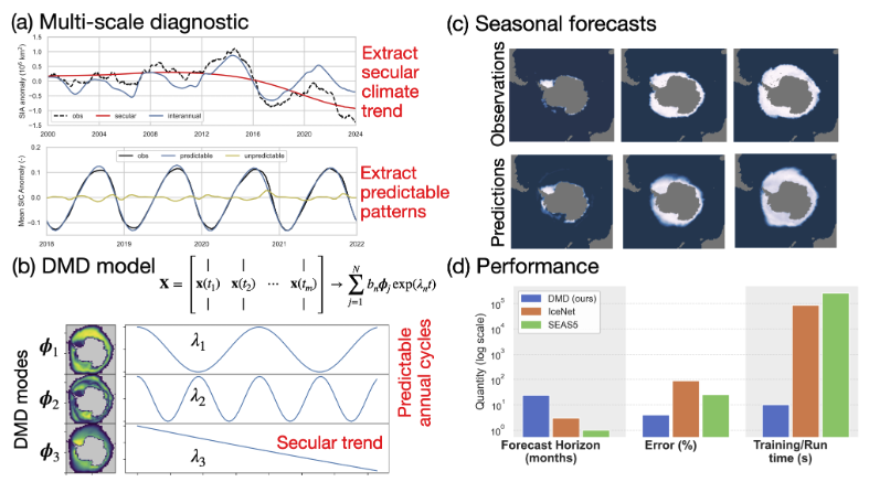
This repository details how to recreate the Figures from the manuscript "Multiscale decomposition reveals predictable interannual variability and climate trends in Antarctic sea ice loss" DOI.

Requirements

• Python: 3.10+ (managed via conda — see environment.yml)
• RAM: 8 GB minimum for figure generation from precomputed results; 32 GB required for full reproduction (DMD training and precomputation)
• Disk space: ~1.5 GB for precomputed results only; ~24 GB for full raw data reproduction
• OS: Linux or macOS recommended; Windows users should use WSL

Quick start (just the figures)

1. Predictive DMD model

conda env create -f environment.yml
conda activate sic_dmd

Download precomputed_results.pkl from the GitHub Release page and place it in data/. Then run any figure script:

python scripts/script_figure_6.py
python scripts/script_figure_7.py
python scripts/script_figure_8.py

2. mrCOSTS analysis

Run the python script version of the mrCOSTS notebook but first set the fit flag (line 158) to be True. Then it can be run as:

python mrCOSTS\ analysis/ice-dmd_mrcosts-figs.py

3. Results

Output of all scripts appears in figures/.

Full reproduction from raw data

1. Obtain the data

Download the files listed below and place them under data/:

File	Size	Source
ice_conc_sh_ease2-250_icdr-v2p0_*.nc	5.7MB per day	OSI-SAF v2.0 (DOI)
Antarctic_years_1989_2024i.pkl	22 GB	Zenodo (DOI) (post-processed)
DMD_r_5_day_34_0_thin_2_win_7.pkl	616 MB	GitHub Release (upload in progress)
precomputed_results.pkl	1.3 GB	GitHub Release (upload in progress)
coarsened-15day.all-years.v2024-09-20.nc	36 MB	Github
land-mask.nc	1.5 MB	Github

Note: The OSI SAF observation data is temporarily hosted on Dropbox via the link above. We will soon upload all data files to Zenodo and Hugging Face for permanent archival.

The precomputed file is enough to generate all predictive DMD figures. Both DMD_r_5_day_34_0_thin_2_win_7.pkl and precomputed_results.pkl can be regenerated from the raw observations using train_dmd.py and precompute.py (see steps 2–3 below).

The coarsened-15day.all-years.v2024-09-20.nc and land-mask files are for the mrCOSTS analysis. The original data were coarsened to 150 km x 150 km grids and 15 day averages since the high-frequency, high spatial resolution components of the system were not targetted. The land mask simply masks the location of Antarctica.

2. Train predictive DMD model (optional -- skip if you downloaded precomputed_results.pkl)

This loads the raw observations (~22 GB), builds a window-averaged training set, and trains a 100-member bootstrap DMD ensemble via BOPDMD. Requires at least 32 GB of RAM.

python scripts/train_dmd.py

Output: data/DMD_r_5_day_34_0_thin_2_win_7.pkl (~616 MB)

3. Precompute the predictive model (optional -- skip if you downloaded precomputed_results.pkl)

This loads the raw observations and the DMD model from the previous step, evaluates the ensemble on training and prediction windows, computes climatology statistics, and writes data/precomputed_results.pkl. Requires at least 32 GB of RAM.

python scripts/precompute.py

4. Generate predictive DMD model figures

Each script loads the precomputed results and runs in a few seconds:

python scripts/script_figure_6.py     # Total ice coverage prediction
python scripts/script_figure_7.py     # Forecast MAE
python scripts/script_figure_8.py     # Combined spatial maps + probe time series
python scripts/script_figure_s1.py    # Supplementary: 2022 reconstruction
python scripts/script_figure_s2.py    # Supplementary: climatology at probes

5. Generate mrCOSTS Figures

The mrCOSTS analysis is located in notebooks\ice-dmd_mrcosts-figs.ipynb and can be run using the same environment as the predictive DMD model after setting up jupyter. See the data notes above. You will need to make sure the conda environment is visible to jupyter lab.

In order to reproduce the mrCOSTS figures you will need to fit mrCOSTS by setting the fit flag to True.

The script can also be run as

python mrCOSTS\ analysis/ice-dmd_mrcosts-figs.py

Figures

Script	Paper figure	Description
ice-dmd_mrcosts-figs.ipynb	Figure 1	Overview (mrCOSTS components)
ice-dmd_mrcosts-figs.ipynb	Figure 2	Interannual variability (mrCOSTS)
ice-dmd_mrcosts-figs.ipynb	Figure 3	Background mode spatial patterns
ice-dmd_mrcosts-figs.ipynb	Figure 4	mrCOSTS band amplitudes
ice-dmd_mrcosts-figs.ipynb	Figure 5	mrCOSTS point diagnosis
script_figure_6.py	Figure 6	Total ice coverage: DMD vs climatology
script_figure_7.py	Figure 7	Mean absolute error of DMD forecast
script_figure_8.py	Figure 8	Observed vs predicted SIC maps + probe time series
script_figure_s1.py	Suppl. S1	DMD reconstruction quality (2022)
script_figure_s2.py	Suppl. S2	Climatology vs 2023 at probe locations

Repository structure

src/sic_dmd/           Python package with shared utilities
  config.py            All parameters, paths, and constants
  data_wrangle.py      Data loading, thinning, leap-year removal
  dmd_routines.py      DMD training, evaluation, bootstrap
  plotting.py          Shared plotting helpers (colormaps, maps)
scripts/               One script per figure + DMD training + precompute
data/                  Input data (not tracked in git except those used to fit mrCOSTS)
figures/               Generated figures (not tracked in git)
mrCOSTS analysis/      Notebook and script for performing the mrCOSTS analysis

Citation

If you use this code or data in your work, please cite:

@misc{yatsyshin2026multiscaledecompositionrevealspredictable,
      title={Multiscale Decomposition Reveals Predictable Interannual Variability and Climate Trends in Antarctic Sea Ice Loss}, 
      author={Peter Yatsyshin and Karl Lapo and Oliver Strickson and Louisa van Zeeland and J. Scott Hosking and J. Nathan Kutz},
      year={2026},
      eprint={2604.26594},
      archivePrefix={arXiv},
      primaryClass={physics.ao-ph},
      url={https://arxiv.org/abs/2604.26594}, 
}