

![]()

Note
{wbw} is currently in alpha. Expect breaking changes both in the API and in outputs.
The {wbw} package provides R bindings for the Whitebox Workflows for Python — a powerful and fast library for advanced geoprocessing, with focus on hydrological, geomorphometric and remote sensing analysis of raster, vector and LiDAR data.
The {wbw} R package introduces several new S7 classes, including
WhiteboxRaster and WhiteboxVector which serves as a bridge between
Python and R.
library(wbw)

raster_path <- system.file("extdata/dem.tif", package = "wbw")
dem <- wbw_read_raster(raster_path)
dem
#> +------------------------------------------+
#> | WhiteboxRaster                           |
#> | dem.tif                                  |
#> |..........................................|
#> | bands       : 1                          |
#> | dimensions  : 726, 800  (nrow, ncol)     |
#> | resolution  : 5.002392, 5.000243  (x, y) |
#> | EPSG        : 2193  (Linear_Meter)       |
#> | min value   : 63.698193                  |
#> | max value   : 361.020721                 |
#> +------------------------------------------+
The true power of {wbw} unleashes when there’s a need to run several
operations sequentially, i.e., in a pipeline. Unlike the original
Whitebox Tools, WbW stores files in
memory,
reducing the amount of intermediate I/O operations.
For example, a DEM can be smoothed (or filtered), and then the slope can be estimated as follows:
dem |>
  wbw_mean_filter() |>
  wbw_slope(units = "d")
#> +------------------------------------------+
#> | WhiteboxRaster                           |
#> | Slope (degrees)                          |
#> |..........................................|
#> | bands       : 1                          |
#> | dimensions  : 726, 800  (nrow, ncol)     |
#> | resolution  : 5.002392, 5.000243  (x, y) |
#> | EPSG        : 2193  (Linear_Meter)       |
#> | min value   : 0.005972                   |
#> | max value   : 50.069439                  |
#> +------------------------------------------+The above example may remind you of the {terra} package, and it is not
a coincidence. The {wbw} package is designed to be fully compatible
with {terra}, and the conversion between WhiteboxRaster and
SpatRaster objects happens in milliseconds (well, depending on the
raster size, of course).
library(terra)

wbw_read_raster(raster_path) |>
  wbw_gaussian_filter(sigma = 1.5) |>
  wbw_aspect() |>
  as_rast() |> # Conversion to SpatRaster
  plot(main = "Aspect")
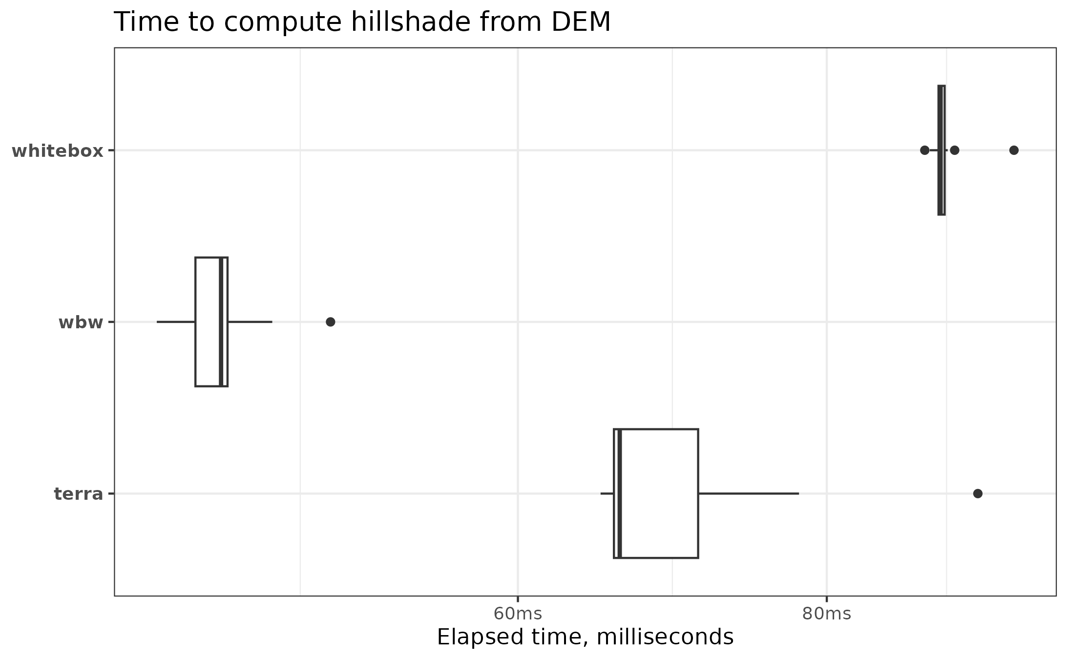
The {wbw} package is quite fast; you can see the detailed benchmarks here. In most cases, it is as fast as terra, while excelling in some more complex tasks (such as hillshading and filtering). Additionally, wbw outperforms the original {whitebox} by 2 to 3 times, as the amount of I/O operations is reduced to a minimum.
You can install the development version of {wbw} from
GitHub with:
# install.packages("pak")
pak::pak("atsyplenkov/wbw")
Tip
The {wbw} package requires the whitebox-workflows Python library
v1.3.3+. However, you should not worry about it, as the package
is designed to install all dependencies automatically on the first run.
Your machine should have Python 3.8+ installed with pip and venv configured. Usually, these requirements are met on all modern computers. However, clean Debian installs may require the installation of system dependencies:
apt update
apt install python3 python3-pip python3-venv -yContributions are welcome! Please see our contributing
guidelines for details. There is an open issue for the
{wbw} package here that
contains a list of functions yet to be implemented. This is a good place
to start.
Geomorphometric and hydrological analysis in R can be also done with:
{whitebox}— An R frontend for the WhiteboxTools standalone runner.{traudem}— R bindings to TauDEM (Terrain Analysis Using Digital Elevation Models) command-line interface.{RSagacmd}and{RSAGA}— Links R with SAGA GIS.{rivnet}— river network extraction from DEM using TauDEM.