In this notebook I will respond and discuss the following points:
It is a Python package, specialized for building and manipulating large and multidimensional arrays. NumPy has built-in functions for linear algebra and random number generation. It is an important library because many of the other Python packages such as SciPy, Matplotlib rely on Numpy to work (to a reasonable degree).
The numpy.random module supplements Python's built-in random with functions to efficiently generate complete arrays of sample values from many types of probability distributions. Python source for data analysis by Wes McKinney.
import numpy as np
import matplotlib.pyplot as plt
import pandas as pd
import seaborn as sns
from matplotlib.ticker import FuncFormatter
To begin with, we’ll first import the NumPy module by running import numpy as np, allowing us to access all relevant functions in the module.
import numpy as np
This method generates random numbers in a given shape. Some common examples are given below. Note that the numbers specified in the rand() function correspond to the number of dimensions of the array that is to be generated. A special case is that when no numbers are specified in the function, a random value will be generated.
np.random.rand()
0.5242129213883749
np.random.rand(4)
array([[0.27452013, 0.4426765 , 0.23433773, 0.86329531],
   `[0.02179784, 0.23914946, 0.24846379, 0.41607698],`

   `[0.3212738 , 0.37238859, 0.43868957, 0.30780613]])`
Both methods are used to generate random numbers from the standard normal distribution, the curves of which are shown in the figure below. The red curve shows you the standard normal distribution with a mean of 0 and standard deviation of 1.

standard_normal() method, we need to use a tuple to set the shape size. Some common examples are given below.
np.random.randn(4)
In the file 1. Random numbers in NumPy.ipynb we develop and explain in detail the Numpy random numbers.
In this section we will develop the Simple Random Data function and generate random numbers of different types, such as matrices of various shapes, normally distributed matrices, ranges of floats of different parameters such as the range, dimensions and probabilities of the returned values.
The following lines of code demonstrate the usefulness of the random.rand function to generate random numbers between 0 and 1 and how this data can then be manipulated, plotted and visualised.
#returns array of random floats between 0 and 1 of shape (d0 to dn)
import numpy as np #import numpy package
import matplotlib.pyplot as plt
import scipy as sc
from scipy import stats
import math as mt
import pandas as pd
%matplotlib inline
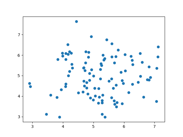
R1 = np.random.rand(100,1) #return 100 x 1 random array of floats between 0 and (not including) 1
x = np.arange(100) #create a list 0f 1 to 100 in order to plot the random no's created against in a scatter plot
plt.scatter(x,R1)
plt.title("plot of 100 random floats ")
Text(0.5, 1.0, 'plot of 100 random floats ')
The Permutations functions, shuffle and permutation both generate random numbers with the shuffle function changing the order of a given set of inputs. The permutation function will create a random sequence of numbers given an input length.
The following code creates a lotto draw using the shuffle function
i = list(range(1, 43)) #create a list of 42 numbers
x = np.array(i) #convert to a numpy array
np.random.shuffle(x) #shuffle the numbers
x
draw = x[0:6] #output first 6 random numbers
'The lotto numbers are', draw # dispay the lotto numbers
('The lotto numbers are', array([ 3, 42, 12, 21, 20, 14]))
Example of the use of the permutation function to create a random password
#A small example of how the permutation function can be used to generate a random password
Letters = np.array(['A', 'B', 'C', 'D', 'E', 'F', 'G', 'H', 'I', 'J', 'K', 'L', 'M', 'N', 'O', 'P', 'Q', 'R', 'S', 'T', 'U', 'V', 'X', 'Y', 'Z'])
Order = np.random.permutation(Letters)
print('Password is =', Order[1:7])
Password is = ['R' 'E' 'I' 'C' 'V' 'T']
The file 2.Simple random data and Permutations.ipynb demonstrates the utility of the random.rand function to generate random numbers between 0 and 1 and how this data can be manipulated, plotted, and displayed.
The data distribution is a list of all possible values and the frequency with which each value occurs. These lists are important when working with statistics and data science.
The random module offers methods that return randomly generated data distributions.
Normal distributions are often used in the natural and social sciences to represent real-valued random variables whose distributions are not known. The normal distribution is a continuous theoretical probability distribution.
In the previous chapter we learned how to create a completely random array, of a given size, and between two given values.
In this chapter we will learn how to create an array where the values are concentrated around a given value.
In probability theory this kind of data distribution is known as the normal data distribution, or the Gaussian data distribution, after the mathematician Carl Friedrich Gauss who came up with the formula of this data distribution.
A typical normal data distribution:
import matplotlib.pyplot as plt

x = numpy.random.normal(5.0, 1.0, 100000)

plt.hist(x, 100)
plt.show()
Result:
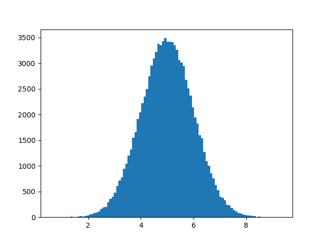
Nota: Un gráfico de distribución normal también se conoce como curva de campana debido a su forma característica de campana.
We use the array from the numpy.random.normal() method, with 100000 values, to draw a histogram with 100 bars.
We specify that the mean value is 5.0, and the standard deviation is 1.0.
Meaning that the values should be concentrated around 5.0, and rarely further away than 1.0 from the mean.
And as you can see from the histogram, most values are between 4.0 and 6.0, with a top at approximately 5.0.
A scatter plot is a diagram where each value in the data set is represented by a dot.
The Matplotlib module has a method for drawing scatter plots, it needs two arrays of the same length, one for the values of the x-axis, and one for the values of the y-axis:
x = [5,7,8,7,2,17,2,9,4,11,12,9,6]

y = [99,86,87,88,111,86,103,87,94,78,77,85,86]
The x array represents the age of each car.
The y array represents the speed of each car.
Use the scatter() method to draw a scatter plot diagram:
import matplotlib.pyplot as plt

x = [5,7,8,7,2,17,2,9,4,11,12,9,6]
y = [99,86,87,88,111,86,103,87,94,78,77,85,86]

plt.scatter(x, y)
plt.show()
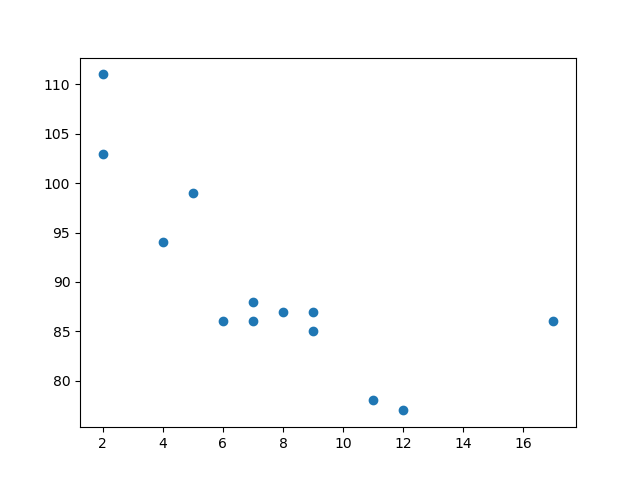
The x-axis represents ages, and the y-axis represents speeds.
What we can read from the diagram is that the two fastest cars were both 2 years old, and the slowest car was 12 years old.
Note: It seems that the newer the car, the faster it drives, but that could be a coincidence, after all we only registered 13 cars.
In Machine Learning the data sets can contain thousands-, or even millions, of values.
You might not have real world data when you are testing an algorithm, you might have to use randomly generated values.
As we have learned in the previous chapter, the NumPy module can help us with that!
Let us create two arrays that are both filled with 1000 random numbers from a normal data distribution.
The first array will have the mean set to 5.0 with a standard deviation of 1.0.
The second array will have the mean set to 10.0 with a standard deviation of 2.0:
A scatter plot with 1000 dots:
import numpy
import matplotlib.pyplot as plt

x = numpy.random.normal(5.0, 1.0, 1000)
y = numpy.random.normal(10.0, 2.0, 1000)

plt.scatter(x, y)
plt.show()
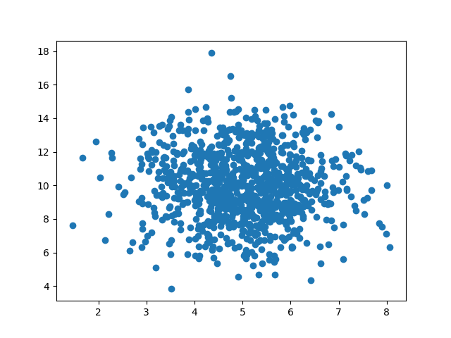
We can see that the dots are concentrated around the value 5 on the x-axis, and 10 on the y-axis.
We can also see that the spread is wider on the y-axis than on the x-axis.
The 3.Distributions funtions.ipynb file explains the use and purpose of at least five "Distributions" functions.
The use of randomness is an important part of configuring and evaluating machine learning algorithms.
From randomly initializing weights in an artificial neural network to dividing data into test sets and random trains, shuffling a set of stochastic gradient descent training data, generating random numbers, and taking advantage of randomness is a skill. necessary.
The source of randomness that we inject into our programs and algorithms is a mathematical trick called a pseudorandom number generator.
A random number generator is a system that generates random numbers from a true source of randomness. Often something physical, such as a Geiger counter, where the results are turned into random numbers. We do not need true randomness in machine learning. Instead we can use pseudorandomness. Pseudorandomness is a sample of numbers that look close to random, but were generated using a deterministic process.
Shuffling data and initializing coefficients with random values use pseudorandom number generators. These little programs are often a function that you can call that will return a random number. Called again, they will return a new random number. Wrapper functions are often also available and allow you to get your randomness as an integer, floating point, within a specific distribution, within a specific range, and so on.
The numbers are generated in a sequence. The sequence is deterministic and is seeded with an initial number. If you do not explicitly seed the pseudorandom number generator, then it may use the current system time in seconds or milliseconds as the seed.
The value of the seed does not matter. Choose anything you wish. What does matter is that the same seeding of the process will result in the same sequence of random numbers.
The Python standard library provides a module called random that offers a suite of functions for generating random numbers.
Python uses a popular and robust pseudorandom number generator called the Mersenne Twister.
In this section, we will look at a number of use cases for generating and using random numbers and randomness with the standard Python API.
Seed The Random Number Generator The pseudorandom number generator is a mathematical function that generates a sequence of nearly random numbers.
It takes a parameter to start off the sequence, called the seed. The function is deterministic, meaning given the same seed, it will produce the same sequence of numbers every time. The choice of seed does not matter.
The seed() function will seed the pseudorandom number generator, taking an integer value as an argument, such as 1 or 7. If the seed() function is not called prior to using randomness, the default is to use the current system time in milliseconds from epoch (1970).
The example below demonstrates seeding the pseudorandom number generator, generates some random numbers, and shows that reseeding the generator will result in the same sequence of numbers being generated.
# seed the pseudorandom number generator
from random import seed
from random import random
# seed random number generator
seed(1)
# generate some random numbers
print(random(), random(), random())
# reset the seed
seed(1)
# generate some random numbers
print(random(), random(), random())
0.13436424411240122 0.8474337369372327 0.763774618976614
0.13436424411240122 0.8474337369372327 0.763774618976614
Running the example seeds the pseudorandom number generator with the value 1, generates 3 random numbers, reseeds the generator, and shows that the same three random numbers are generated.
It can be useful to control the randomness by setting the seed to ensure that your code produces the same result each time, such as in a production model.
For running experiments where randomization is used to control for confounding variables, a different seed may be used for each experimental run.
File 4. Using seeds to generate pseudorandom numbers.ipynb explains the use of seeds to generate pseudorandom numbers.
Series:Community Experience Distilled Authors: Rossant, Cyrille Publication Information: Ed.: Second edition. Birmingham, UK : Packt Publishing. 2015 Resource Type: eBook
IPython Interactive Computing and Visualization Cookbook : Over 100 Hands-on Recipes to Sharpen Your Skills in High-performance Numerical Computing and Data Science in the Jupyter Notebook, 2nd Edition
Series:Community Experience Distilled Authors: Rossant, Cyrille Publication Information: Ed.: Second edition. Birmingham : Packt Publishing. 2018 Resource Type: eBook
Hands-On Data Analysis con NumPy y pandas: Implementar Python Paquetes De Datos manipulación para procesamiento
Authors: Miller, Curtis Publication Information: Birmingham: Packt Publishing. 2018 Resource Type: eBook
Series:Community Experience Distilled Authors: Idris, Ivan Publication Information: Birmingham, U.K. : Packt Publishing. 2014 Resource Type: eBook
Authors: Fandango, Armando Publication Information: Ed.: Second edition. Birmingham : Packt Publishing. 2017 Resource Type: eBook