Docs	Paper	Slides	Colab	pip	conda

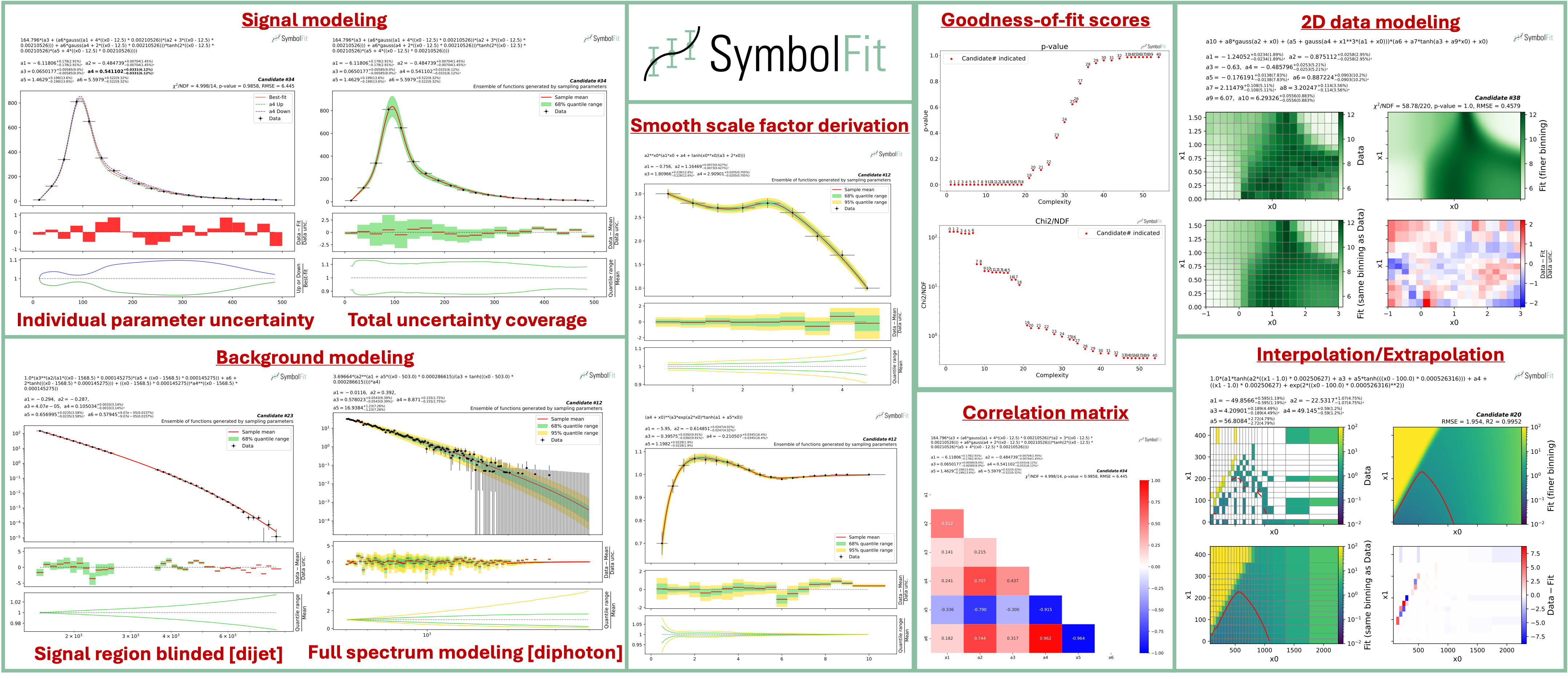
An API to automate parametric modeling with symbolic regression, originally developed for data analysis in the experimental high-energy physics community, but also applicable beyond.

SymbolFit takes binned data with measurement/systematic uncertainties (optional) as input, utilizes PySR to perform a machine-search for batches of functional forms that model the data, parameterizes these functions, and utilizes LMFIT to re-optimize the functions and provide uncertainty estimation, all in one go. It is designed to maximize automation with minimal human input. Each run produces a batch of functions with uncertainty estimation, which are evaluated, saved, and plotted automatically into readable output files, ready for downstream tasks.

In short, symbolfit = pysr (symbolic regression to generate functional forms) + lmfit (re-optimization & uncertainty modeling) + auto-evaluation tools (parameter correlation, uncertainty variation and coverage, statistical tests, etc.).

• Installation
• Getting Started
• Documentation
• Citation

Installation

Installation via PyPI

With python>=3.10 and pip:

pip install symbolfit

Installation via conda

conda create --name symbolfit_env python=3.10
conda activate symbolfit_env
conda install -c conda-forge symbolfit

Julia (backend for PySR) will be automatically installed at first import of PySR:

import pysr

Getting Started

To run an example fit, get the example datasets by cloning this repo:

git clone https://github.com/hftsoi/symbolfit.git
cd symbolfit

Then within a python session (or simply do python fit_example.py):

from symbolfit.symbolfit import *

dataset = importlib.import_module('examples.datasets.toy_dataset_1.dataset')
pysr_config = importlib.import_module('examples.pysr_configs.pysr_config_gauss').pysr_config

model = SymbolFit(
    	x = dataset.x,
    	y = dataset.y,
    	y_up = dataset.y_up,
    	y_down = dataset.y_down,
    	pysr_config = pysr_config,
    	max_complexity = 60,
    	input_rescale = True,
    	scale_y_by = 'mean',
    	max_stderr = 20,
    	fit_y_unc = True,
    	random_seed = None,
    	loss_weights = None
)

model.fit()

After the fit, save results to csv files:

model.save_to_csv(output_dir = 'output_dir/')

and plot results to pdf files:

model.plot_to_pdf(
    	output_dir = 'output_dir/',
    	bin_widths_1d = dataset.bin_widths_1d,
    	plot_logy = False,
    	plot_logx = False,
        sampling_95quantile = False,
        #bin_edges_2d = dataset.bin_edges_2d,
        #plot_logx0 = False,
        #plot_logx1 = False,
        #cbar_min = None,
        #cbar_max = None,
        #cmap = None,
        #contour = None,
        # ^ additional options for 2D plotting
)

Candidate functions with full substitutions can be printed promptly:

model.print_candidate(candidate_number = 20)

When preparing for your own data, a graphical illustration of the input data format can be found here.

Each fit will produce a batch of candidate functions and will automatically save all results to six output files:

1. candidates.csv: saves all candidate functions and evaluations in a csv table.
2. candidates_compact.csv: saves a reduced version for essential information without intermediate results.
3. candidates.pdf: plots all candidate functions (1D/2D only for now) with associated uncertainties one by one for fit quality evaluation.
4. candidates_sampling.pdf: plots all candidate functions (1D only for now) with total uncertainty coverage generated by sampling parameters.
5. candidates_gof.pdf: plots the goodness-of-fit scores.
6. candidates_correlation.pdf: plots the correlation matrices for the parameters of the candidate functions.

Output files from an example fit can be found and downloaded here for illustration.

Note: The function space is usually huge, even when constrained by the pysr config. This means that if you are not satisfied with the results from a fit, you can simply rerun it with the exact same config and obtain a completely different set of candidate functions—the only difference being the random seed that initiates the seeding functions. Therefore, you can rerun the fit as many times as you want until you are satisfied with the results. If you use model = SymbolFit(..., random_seed = None, ...), nothing needs to be changed—just rerun the fit. If you set a specific random_seed, change its value before rerunning. However, if you are still not satisfied with the results after many trials, it might indicate an issue with the config. Then you might want to try a different config, tune it, and start new runs.

For detailed instructions and more demonstrations, please check out the Colab notebook and the documentation.

Documentation

The documentation can be found here for more information and demonstrations.

Citation

If you find this useful in your research, please consider citing both SymbolFit PySR:

@article{Tsoi:2024pbn,
    author = "Tsoi, Ho Fung and Rankin, Dylan and Caillol, Cecile and Cranmer, Miles and Dasu, Sridhara and Duarte, Javier and Harris, Philip and Lipeles, Elliot and Loncar, Vladimir",
    title = "{SymbolFit: Automatic Parametric Modeling with Symbolic Regression}",
    eprint = "2411.09851",
    archivePrefix = "arXiv",
    primaryClass = "hep-ex",
    doi = "10.1007/s41781-025-00140-9",
    journal = "Comput. Softw. Big Sci.",
    volume = "9",
    pages = "12",
    year = "2025"
}

@misc{cranmerInterpretableMachineLearning2023,
      title = {Interpretable {Machine} {Learning} for {Science} with {PySR} and {SymbolicRegression}.jl},
      url = {http://arxiv.org/abs/2305.01582},
      doi = {10.48550/arXiv.2305.01582},
      urldate = {2023-07-17},
      publisher = {arXiv},
      author = {Cranmer, Miles},
      month = may,
      year = {2023},
      note = {arXiv:2305.01582 [astro-ph, physics:physics]},
      keywords = {Astrophysics - Instrumentation and Methods for Astrophysics, Computer Science - Machine Learning, Computer Science - Neural and Evolutionary Computing, Computer Science - Symbolic Computation, Physics - Data Analysis, Statistics and Probability},
}