torch-fem

Simple GPU accelerated differentiable finite elements for solid mechanics with PyTorch. PyTorch enables efficient computation of sensitivities via automatic differentiation and using them in optimization tasks.

Installation

You may install torch-fem via pip with

pip install torch-fem

Optional: For GPU support, install CUDA, PyTorch for CUDA, and the corresponding CuPy version.

For CUDA 11.8:

pip install torch torchvision torchaudio --index-url https://download.pytorch.org/whl/cu118
pip install cupy-cuda11x # v11.2 - 11.8

For CUDA 12.9:

pip install torch torchvision torchaudio --index-url https://download.pytorch.org/whl/cu129
pip install cupy-cuda12x # v12.x

Features

• Elements

  • 1D: Bar1, Bar2
  • 2D: Quad1, Quad2, Tria1, Tria2
  • 3D: Hexa1, Hexa2, Tetra1, Tetra2
  • Shell: Flat-facet triangle (linear only)

• Material models

  • Isotropic linear elasticity
  • Orthotropic linear elasticity
  • Isotropic small strain plasticity
  • Isotropic small strain damage
  • Hyperelasticity (via automatic differentiation of their energy function)
  • Isotropic thermal conductivity
  • Orthotropic thermal conductivity
  • Custom user material interface

• Utilities

  • Homogenization of orthotropic elasticity for composites
  • Simple structured meshing
  • I/O to and from other mesh formats via meshio

Basic examples

The subdirectory examples/basic contains a couple of Jupyter notebooks demonstrating the use of torch-fem for trusses, planar problems, shells, and solids. You may click on the examples to check out the notebooks online.

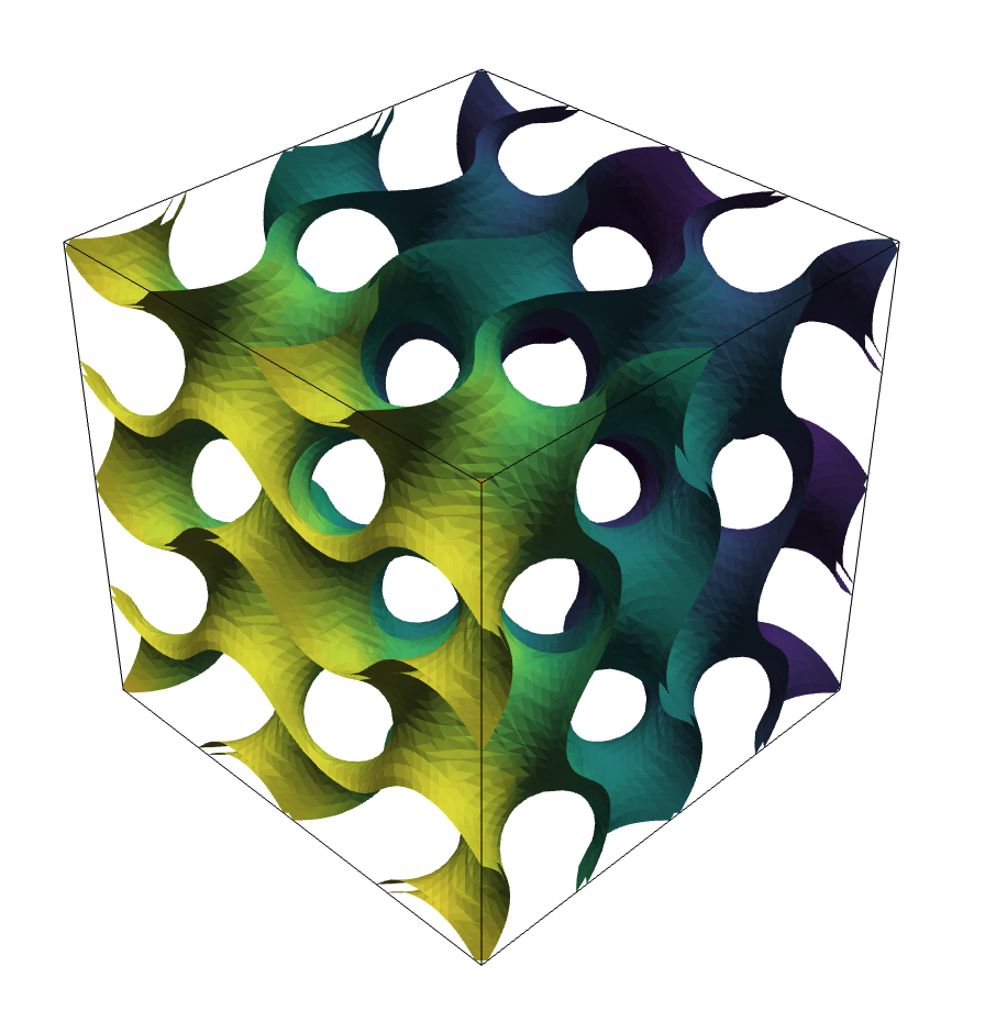
Gyroid: Support for voxel meshes and implicit surfaces.	Solid cubes: There are several examples with different element types rendered in PyVista.	Planar cantilever beams: There are several examples with different element types rendered in matplotlib.
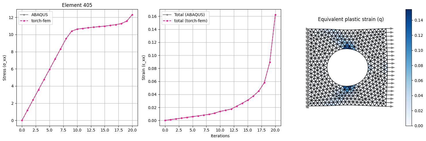
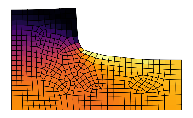
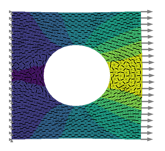
Plasticity in a plate with hole: Isotropic linear hardening model for plane-stress or plane-strain.
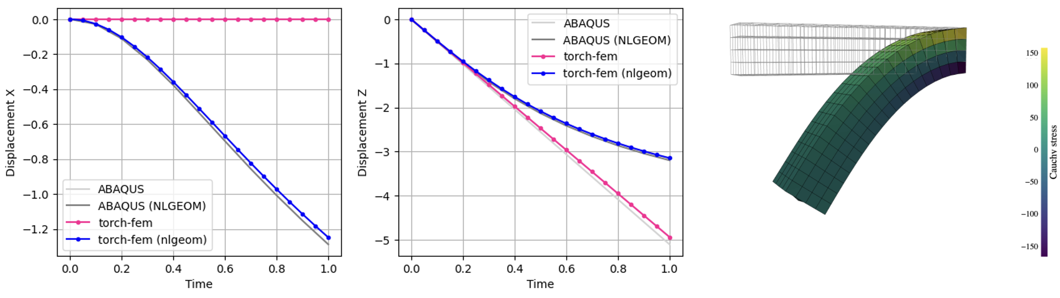
Finite strain cantilever: Hyperelastic model in Total Lagrangian Formulation.

Optimization examples

The subdirectory examples/optimization demonstrates the use of torch-fem for optimization of structures (e.g. topology optimization, composite orientation optimization). You may click on the examples to check out the notebooks online.

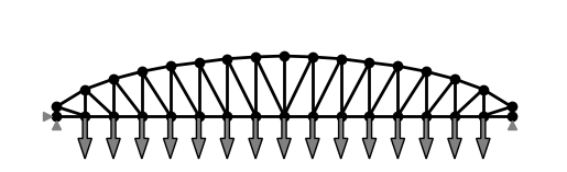
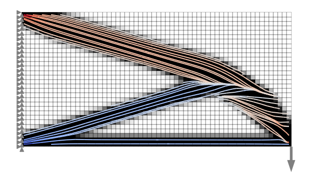
Shape optimization of a truss: The top nodes are moved and MMA + autograd is used to minimize the compliance.	Shape optimization of a fillet: The shape is morphed with shape basis vectors and MMA + autograd is used to minimize the maximum stress.
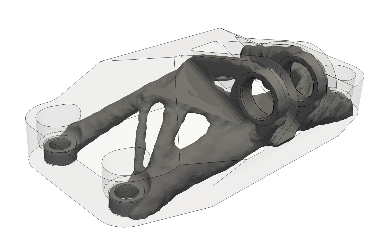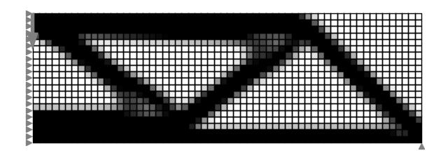
Topology optimization of a MBB beam: You can switch between analytical and autograd sensitivities.	Topology optimization of a jet engine bracket: The 3D model is exported to Paraview for visualization.
Combined topology and orientation optimization: Compliance is minimized by optimizing fiber orientation and density of an anisotropic material using automatic differentiation.	Fiber orientation optimization of a plate with a hole Compliance is minimized by optimizing the fiber orientation of an anisotropic material using automatic differentiation w.r.t. element-wise fiber angles.
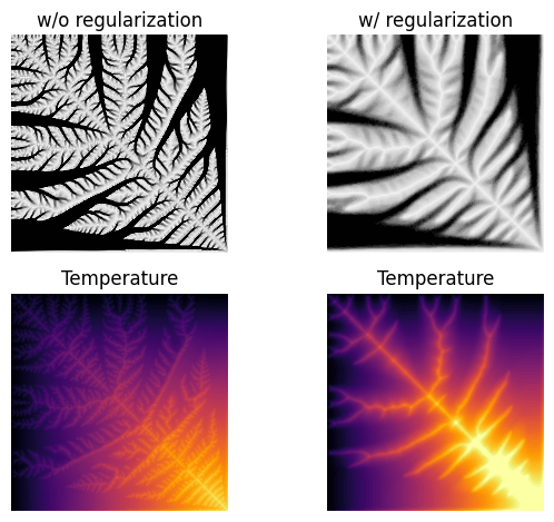
Heat sink: Thermal topology optimization

Minimal example

This is a minimal example of how to use torch-fem to solve a very simple planar cantilever problem.

import torch
from torchfem import Planar
from torchfem.materials import IsotropicElasticityPlaneStress

torch.set_default_dtype(torch.float64)

# Material
material = IsotropicElasticityPlaneStress(E=1000.0, nu=0.3)

# Nodes and elements
nodes = torch.tensor([[0., 0.], [1., 0.], [2., 0.], [0., 1.], [1., 1.], [2., 1.]])
elements = torch.tensor([[0, 1, 4, 3], [1, 2, 5, 4]])

# Create model
cantilever = Planar(nodes, elements, material)

# Load at tip [Node_ID, DOF]
cantilever.forces[5, 1] = -1.0

# Constrained displacement at left end [Node_IDs, DOFs]
cantilever.constraints[[0, 3], :] = True

# Show model
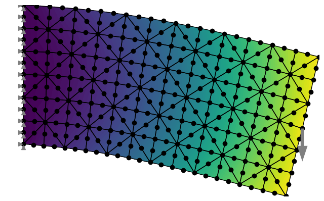
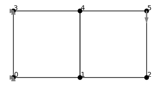
cantilever.plot(node_markers="o", node_labels=True)

This creates a minimal planar FEM model:

# Solve
u, f, σ, F, α = cantilever.solve()

# Plot displacement magnitude on deformed state
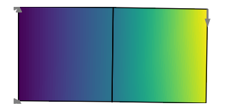
cantilever.plot(u, node_property=torch.norm(u, dim=1))

This solves the model and plots the result:

If we want to compute gradients through the FEM model, we simply need to define the variables that require gradients. Automatic differentiation is performed through the entire FE solver. Rather than differentiating through individual solver iterations or Newton iterations (this would explode in memory and autograd graph size) though, the implicit function theorem is used to formulate an adjoint backward for solve().

# Enable automatic differentiation
cantilever.thickness.requires_grad = True
u, f, _, _, _ = cantilever.solve(differentiable_parameters=cantilever.thickness)

# Compute sensitivity of compliance w.r.t. element thicknesses
compliance = torch.inner(f.ravel(), u.ravel())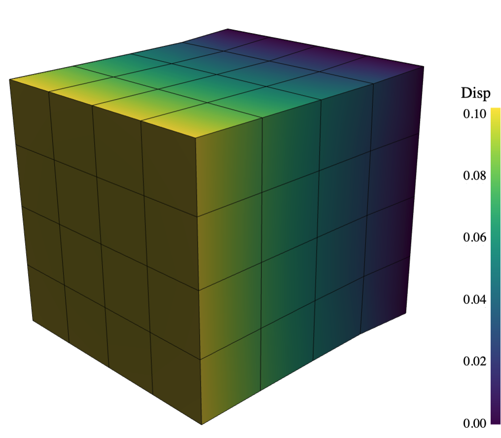
torch.autograd.grad(compliance, cantilever.thickness)[0]

Benchmarks

The following benchmarks were performed on a cube subjected to a one-dimensional extension. The cube is discretized with N x N x N linear hexahedral elements, has a side length of 1.0 and is made of a material with Young's modulus of 1000.0 and Poisson's ratio of 0.3. The cube is fixed at one end and a displacement of 0.1 is applied at the other end. The benchmark measures the forward time to assemble the stiffness matrix and the time to solve the linear system. In addition, it measures the backward time to compute the sensitivities of the sum of displacements with respect to forces.

Apple M1 Pro (10 cores, 16 GB RAM)

Python 3.10, SciPy 1.15.3, Apple Accelerate, float64

N	DOFs	Setup	FWD Solve	BWD Solve	Peak RAM
10	3000	0.02s	0.16s	0.37s	490.4MB
20	24000	0.14s	0.74s	0.35s	895.6MB
30	81000	0.52s	2.73s	0.84s	1947.5MB
40	192000	1.23s	6.53s	1.57s	3060.2MB
50	375000	2.63s	13.02s	3.22s	4398.7MB
60	648000	4.71s	26.17s	5.48s	5789.2MB
70	1029000	9.18s	46.37s	9.43s	7893.5MB
80	1536000	13.90s	73.41s	17.95s	9739.0MB

NVIDIA GeForce RTX 5090 (21,760 Cuda cores, 32 GB VRAM)

Python 3.13, CuPy 14.0.1, CUDA 12.9, float64

N	DOFs	Setup	FWD Solve	BWD Solve	Peak RAM
10	3000	0.27s	0.45s	0.46s	1682.9MB
20	24000	0.24s	0.49s	0.49s	1703.6MB
30	81000	0.25s	0.60s	0.59s	1707.4MB
40	192000	0.25s	0.78s	0.73s	1738.4MB
50	375000	0.28s	1.08s	0.94s	1710.4MB
60	648000	0.32s	1.54s	1.27s	1710.8MB
70	1029000	0.39s	2.13s	1.73s	1728.7MB
80	1536000	0.49s	3.76s	3.22s	2220.5MB

Alternatives

There are many alternative Python FEM tools that you may also consider, depending on your needs:

• General-purpose FEM/PDE frameworks
  • FEniCSx (DOLFINx)
  • SfePy
  • scikit-fem
  • FElupe
  • Nutils
• Differentiable or adjoint-capable FEM
  • JAX-FEM
  • dolfin-adjoint
  • PyTorch-FEA