NumPy Neural Network (From Scratch): MNIST Digit Recognizer

A complete, end-to-end Multi-Layer Perceptron (MLP) built entirely from scratch using pure linear algebra and calculus in NumPy. No TensorFlow, no PyTorch, no black boxes.

This project trains a 2-layer deep neural network on the MNIST dataset to recognize handwritten digits and includes a live OpenCV webcam pipeline for real-time, real-world inference.

Features

• Zero-Framework Math Engine: Forward propagation, backpropagation (Chain Rule), and gradient descent implemented strictly using numpy.dot() and matrix operations.
• Non-Linear Architecture: 784 Input Nodes -> 128 Hidden Nodes (ReLU) -> 10 Output Nodes (Softmax).
• Decoupled Architecture: Trains the model once, saves the optimized parameters (.npz), and loads them instantly for lightweight inference.
• Live Camera Inference: Uses OpenCV to capture real-time webcam video, applies Gaussian blurring and Otsu's Thresholding, and feeds live frames into the custom neural network.

---

Installation & Setup

1. Clone the repository:

   git clone https://github.com/ssdunit/digit_recog_LogisticReg
   cd digit_recog_LogisticReg
   

2. Create a virtual environment:

   python3 -m venv .venv
   source .venv/bin/activate
   

3. Install the dependencies:

   pip install numpy opencv-python scikit-learn matplotlib

   (Note: scikit-learn is strictly used to fetch the MNIST dataset efficiently, not for model training).

How to Use

This project is broken into three distinct scripts:

1. Train the Brain (model.py)

   Run this first. It downloads the MNIST images, scales them, and trains the weights using Cross-Entropy Loss.

   python3 model.py

   Outputs: A finaldataset.npz file containing the optimized W and b matrices. Achieved 95.69% test accuracy(max).

2. Static Image Checker (checker.py)

   Test the network by using your live camera feed. (Note: If inbuilt webcam not present follow these steps).

   chmod +x ./camera/dependencies.sh
   ./camera/dependencies.sh
   chmod +x ./camera/camerarun.sh
   ./camera/camerarun.sh

   Once it is done we can move on and run

   python3 checker.py
   

   Outputs: Opens a real-time OpenCV window. Draw a digit on white paper with a thick black marker, hold it inside the targeting box, and watch the model predict the number. Press q to quit.

The Math Behind the Code

This network relies entirely on the following mathematical concepts:

1. Forward Pass:

$$Z_1 = X \cdot W_1 + b_1$$ $$A_1 = \max(0, Z_1) \quad \text{(ReLU Activation)}$$ $$Z_2 = A_1 \cdot W_2 + b_2$$ $$A_2 = \text{Softmax}(Z_2)$$

2. Loss Function (Categorical Cross-Entropy)

Calculates the penalty for incorrect predictions by comparing the predicted probabilities ($A^{[2]}$) against the true One-Hot Encoded labels ($Y$):

$$L = - \frac{1}{m} \sum_{i=1}^{m} \sum_{k=1}^{K} Y_{i,k} \log(A^{[2]}_{i,k})$$

3. Backward Pass (Backpropagation)

Uses the Chain Rule of calculus to trace the error backward from the output layer to the exact weights that caused it.

• Output Layer Gradients:

$$dZ^{[2]} = A^{[2]} - Y$$ $$dW^{[2]} = \frac{1}{m} (A^{[1]})^T \cdot dZ^{[2]}$$ $$db^{[2]} = \frac{1}{m} \sum_{\text{rows}} dZ^{[2]}$$

• Hidden Layer Gradients:

$$dZ^{[1]} = (dZ^{[2]} \cdot (W^{[2]})^T) * \text{ReLU}'(Z^{[1]})$$ $$dW^{[1]} = \frac{1}{m} X^T \cdot dZ^{[1]}$$ $$db^{[1]} = \frac{1}{m} \sum_{\text{rows}} dZ^{[1]}$$

4. Optimizer (Standard Gradient Descent)

Updates the weights and biases by stepping in the opposite direction of the gradient, scaled by the learning rate ($\alpha$):

$$W^{[k]} = W^{[k]} - \alpha \cdot dW^{[k]}$$ $$b^{[k]} = b^{[k]} - \alpha \cdot db^{[k]}$$

Architecture & Mathematical Foundations

This network was purposefully designed from scratch to demonstrate the mathematical mechanics of deep learning. Below is the breakdown of the specific algorithms powering the engine.

1. Activation Functions:

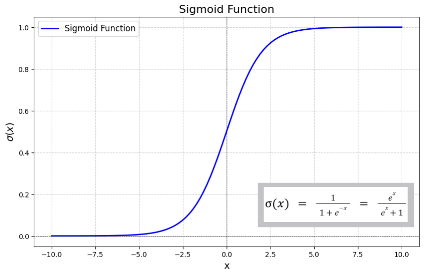
• Sigmoid (The Legacy Function):
  
  

  • Used for hidden layers, it squashes outputs between $0$ and $1$. When chained together, this shrinks the error signal, causing the network to stop learning (The Vanishing Gradient Problem). Clipped to avoid overflow.
  • Formula: $\sigma(z) = \frac{1}{1 + e^{-z}}$
  • Derivative: $\sigma'(z) = \sigma(z)(1 - \sigma(z))$

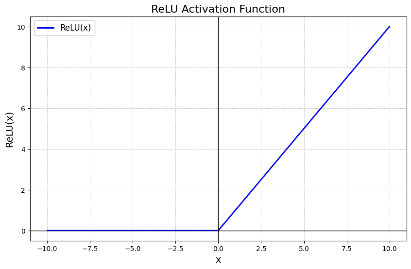
• ReLU (Rectified Linear Unit):
  
  

  • It completely zeroes out negative numbers but passes positive numbers through unchanged. Its derivative is a constant $1$ for all positive values
  • Formula: $f(z) = \max(0, z)$
  • Derivative: $f'(z) = 1 \text{ if } z > 0 \text{ else } 0$

• Softmax (The Output Function): Used strictly in the final layer for multi-class classification. It applies an exponential function to the raw output scores (logits) and divides by the sum of all exponentials. This aggressively amplifies the highest score and forces all 10 output nodes to mathematically compete, ensuring their probabilities perfectly sum to $1.0$ ($100%$ confidence).

  • Formula: $S(z_i) = \frac{e^{z_i}}{\sum_{j=1}^{K} e^{z_j}}$

---

2. The Optimization Engine

The Universal Update Rule (Gradient Descent): $$\theta = \theta - \alpha \nabla J(\theta)$$

• $\theta$ (Parameters): The network's Weights ($W$) and Biases ($b$).
• $\alpha$ (Learning Rate): A scalar determining how large of a "step" the network takes.
• $\nabla J(\theta)$ (Gradient): The multi-dimensional vector pointing up the steepest slope; we subtract it to travel down the curve.
  
  
  
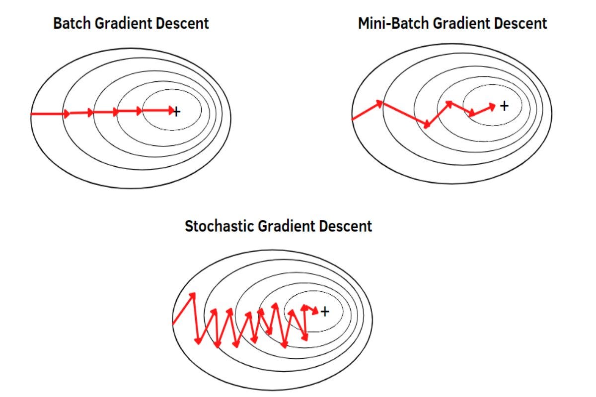
  The Three Strategies:
• Full-Batch Gradient Descent: Feeds all $56,000$ training images into the network at once. It calculates a perfectly smooth, accurate slope. However, it takes massive RAM and easily gets permanently stuck in shallow "fake" valleys (local minima).
• Stochastic Gradient Descent (SGD): Feeds exactly $1$ image at a time. The slope calculation is highly erratic and noisy because it only sees one piece of data. This noise prevents it from getting stuck, but it is incredibly slow to compute in Python and never truly settles at the absolute bottom of the curve. worst algorithm
• Mini-Batch Gradient Descent: The golden compromise. It slices the dataset into shuffled chunks of $128$ images. This introduces just enough mathematical "noise" to bounce the optimizer out of bad valleys, while remaining large enough to take full advantage of NumPy's hyper-fast C-based matrix multiplication. This avoids the issue of the algorithm getting stuck at a shallow point or at a valley of local minima