Learning to Work in the Cloud: JetStream2 and Reproducibility
Important
🕐 Schedule
- 2:00pm-2:10pm: Welcome and Introduction to the topic
- 2:10pm-2:20pm: Getting off your machine (methods for reproducibility)
- 2:20pm-3:00pm: Introducing JetStream2
Important
❗ Requirements
- Basic command line knowledge
- Access to a Terminal
- Unix and Mac users already have access to the Terminal
- Windows users can use either PowerShell or the Windows Subsystem for Linux (WSL)
- A registered CyVerse account (Register for a CyVerse account)
Important
✅ Expected Outcomes
- Reproducibility away from your machine (working in the cloud)
- Knowing where to get compute for research
Earlier in the workshop series we covered aspects of Reproducibility that would allow not only you but your collaborators to access your software in a much quicker and reliable method. These include creating a software environment using Conda and Containers.
Here, we present a summary of these reproducibility methods.
Running a pipeline or a workflow constitutes using a number of different programs, tools and software. Often, these software may run only if of a specific version. To ensure that the pipeline runs, one should specify installing the program/software with the right version.
To help with this, we introduce the use of an Environment Manager called Anaconda (or Conda). An Environment Manager allows you to create software installation directories that are isolated from other installations. You can create unique environments and install specific software version to run specific scripts.
Conda is a popular and open source environment manager tool that can be installed on any operating system (Windows, MacOS, Linux).
Users can create environments that have their own set of packages, dependencies, and even their own version of Python. Another piece of information that's important to remember is that projects can have their own specific requirements, often requiring different versions of the same software. Conda can help you create isolated environments to help softaware not interfering with each other, thus allows for consistent and reproducible results across different systems and setups.
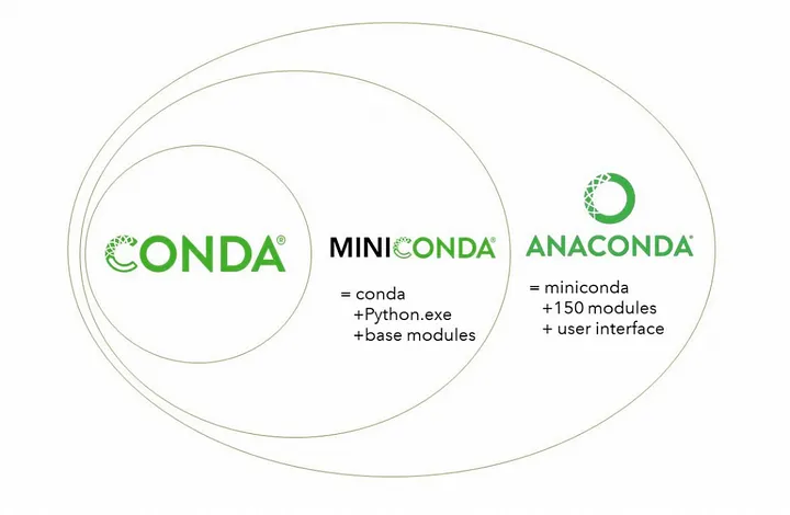
Conda, Miniconda, and Anaconda. Taken from Getting Started with Conda, Medium.

Sharing your scientific analysis code with your colleagues is an essential pillar of Open Science that will help push your field forward.
As disscussed, there are technical challenges that may prevent your colleagues from effectively running your code on their computers, issues related to computing environments.
A solution is to package up the code and all of the software and send it to your colleague as a Container.
A container is a standard unit of software that packages up code and all its dependencies so the application runs quickly and reliably from one computing environment to another
- Container images are a lightweight, standalone, executable package of software that includes everything needed to run an application: code, runtime, system tools, system libraries and settings
- Each of these elements are specifically versioned and do not change
- The recipient does not need to install the software in the traditional sense
A useful analogy is to think of software containers as shipping containers. It allows us move cargo (software) around the world in standard way. The shipping container can be offloading and executed anywhere, as long the destination has a shipping port (i.e., Docker)
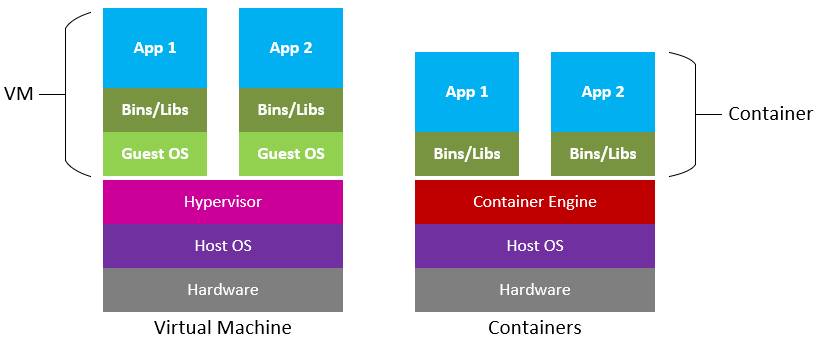
Difference between Virtual Machines and Containers. Containers are a lot more portable as these do not require an OS to be bundled with the software. Figure source: Microsoft Cloudblogs.
Containers are similar to virtual machines (VMs), but are smaller and easier to share. A big distinction between Containers and VMs is what is within each environment: VMs require the OS to be present within the image, whilst containers rely on the host OS and the container engine (e.g., Docker Engine).
Software containers, such as those managed by Docker or Singularity, are incredibly useful for reproducible science for several reasons:
-
Environment Consistency:
- Containers encapsulate the software environment, ensuring that the same versions of software, libraries, and dependencies are used every time, reducing the "it works on my machine" problem.
-
Ease of Sharing:
- Containers can be easily shared with other researchers, allowing them to replicate the exact software environment used in a study.
-
Platform Independence:
- Containers can run on different operating systems and cloud platforms, allowing for consistency across different hardware and infrastructure.
-
Version Control:
- Containers can be versioned, making it easy to keep track of changes in the software environment over time.
-
Scalability:
- Containers can be easily scaled and deployed on cloud infrastructure, allowing for reproducible science at scale.
-
Isolation:
- Containers isolate the software environment from the host system, reducing the risk of conflicts with other software and ensuring a clean and controlled environment.
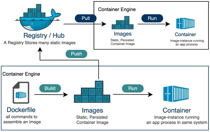
The container's life cycle. Figure source: Tutorialspoint.
Open Science strives to ensure that all science is reproducible, independently from what your machine is. Usually, this allows you to connect to machines and systems that are larger and more powerful than your computer.
However connecting to a machine that isn't yours requires the knowledge of Command Line for connecting, navigating, and executing jobs from a remote location.
Here, we present 2 platforms that allow you to step off your machine and start scaling your research:
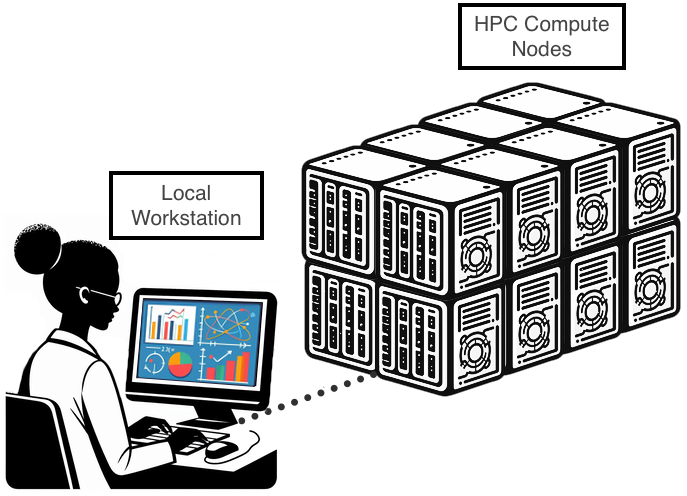
Working at larger US institutions allows for researchers to access High Performance Computing (HPC) resources; The University of Arizona has a powerful HPC platform that faculty, staff and students can access. However, in order to carry out larger submissions, the HPC requires you to be part to approved Projects (usually proposed by a PI).
If you have a UA account, to connect to the HPC you need to use ssh (Secure Shell). Open a terminal, and type:
ssh <UA username>@hpc.arizona.edu
Type your UA password and if successful you'll be greeted with a two-factor login. Select which choice, and complete the authentification. Once you are past the authentification steps, you will enter the Bastion server. This step has 2 purposes:
- Protect from attacks.
- Select what HPC system you want to use.
Note
The Bastion server is NOT YET the HPC! Here you cannot submit jobs or run analyes. Type shell in order to select what system you want to use.
Here are some of the statistics regarding the 3 HPC systems at the UA HPC.
| System | Year of Aquisition | Processors | RAM | GPU |
|---|---|---|---|---|
| Puma | 2020 | 2x AMD Zen2 48 CPU (94 cores total) | 512GB | 6x Nvidia V100S |
| Ocelote | 2016 | 2x Xeon E5-2695v3 14-core (28 cores total) | 192GB | 46x Nvidia P100 |
| El Gato | 2013 | 2x Xeon E5-2650v2 8-core (16 core total) | 64GB | removed as obsolete |
One can find the full systems specs at the official UA HPC documentatio resources page.
El Gato is the oldest system, and potentially not useful for heavy research. Puma is the newest and most requested, whislt Ocelote is the "middle child": not as popular but still able to pack a punch.
Depending on what your work is, your best bet would be Puma for heavy computation (if you are ok with waiting long queues); However, if your jobs aren't as taxing, then Ocelote could easily be a safe choice.
All of the UA HPC systems run on a workload manager and job scheduler named SLURM (Simple Linux Utility for Resource Management). It's designed to manage and schedule computing resources such as CPUs, GPUs, memory, and storage across a cluster of interconnected nodes.
You can learn more on SLURM and HPC system commands here.
There are 2 ways one can submit jobs onto the HPC system. The first is to run a batch job, which is the more popular submission type, whilst the other is by requesting an interactive node.
As we are not going to be using batch submissions, we are not going to be going into too much detail. However, here is what you need to know. For more details on running batch jobs, visit the official documentation page on batch jobs.
Batch scripts require a number of job directives. These are similar to the Dockerfile instructions, but instead of telling Docker how to build the image, these instead tell the SLURM system what to do with the job. The essential directives are the following:
| Directive | Purpose |
|---|---|
#SBATCH --account=group_name |
Specify the account where hours are charged. |
#SBATCH --partition=partition_name |
Set the job partition. This determines your job's priority and the hours charged. |
#SBATCH --time=DD-HH:MM:SS |
Set the job's runtime limit in days, hours, minutes, and seconds. A single job cannot exceed 10 days or 240 hours. |
#SBATCH --nodes=N |
Allocate N nodes to your job. |
#SBATCH --cpus-per-task=M and #SBATCH --ntasks=N
|
ntasks specifies the number of tasks (or processes) the job will run. By default, you will be allocated one CPU/task. This can be increased by including the additional directive --cpus-per-task. |
#SBATCH --mem=Ngb |
Select N gb of memory per node. If "gb" is not included, this value defaults to MB. |
After setting your directives, you can instruct the HPC to do what you require similar to a bash script.
Here's an example of a batch job:
#!/bin/bash
#SBATCH --job-name=blast_job          # Job name
#SBATCH --partition=standard          # Sets the job priority to standard
#SBATCH --nodes=1                     # Number of nodes
#SBATCH --ntasks=1                    # Number of tasks (processes) per node
#SBATCH --cpus-per-task=4             # Number of CPU cores per task
#SBATCH --mem=8G                      # Memory per node (in this case, 8GB)
#SBATCH --time=02:00:00               # Time limit (HH:MM:SS)

# Load necessary modules
module load blast/2.12.0              # Load BLAST module (adjust version as needed)

# Change to the directory where the job will run
cd $SLURM_SUBMIT_DIR

# Define input and output files
query_file="query.fasta"              # Input query file (FASTA format)
database_file="database.fasta"        # BLAST database file (FASTA format)
output_file="blast_results.out"       # Output file for BLAST results

# Run BLAST command
blastp -query $query_file -db $database_file -out $output_file -evalue 0.001 -num_threads $SLURM_CPUS_PER_TASK
- To submit jobs you need to use
sbatch, such assbatch script.slurm - To cancel your job you do
scancel, such asscancel $JOBIDorscancel -u $NETID
This will submit your job to the queue. Execution will depend on your submission type (partition).
An interactive node, unlike batch jobs which are run asynchronously, allows immediate access to compute. Similar to batch jobs, interactive nodes are submitted to the queue, but once available, you will receive a prompt for a node with the selected resources. Read more on how to launch interactive jobs in the official documentation.
Tip
The "Quick and Dirty"
Don't need a lot of resources and just want access to the compute?
Just type interactive.
Disclaimer: you may require to wait longer as your job is going to fall in the windfall queue.
Following are a list of useful flags (options) for setting up the interactive node.
| Flag | Default value | Description | Example |
|---|---|---|---|
-n |
1 | Number of CPUs requested per node | interactive -n 8 |
-m |
4GB | Memory per CPU | interactive -m 5GB |
-a |
none | Account (group) to charge | interactive -a datalab |
--partition= |
windfall | Partition to determine CPU time charges and is set to windfall when no account is specified, and is set to standard when an account is provided. | interactive --partition=windfall |
-t |
01:00:00 | Time allocated to session. | interactive -t 08:00:00 |
-N |
1 | Number of nodes. | There is no reason to exceed 1 node unless the number of CPUs requested is greater than the number of CPUs per node on a given cluster. |
An example for an interactive node is:
interactive -n 8 -m 16GB -a datalab -t 02:00:00
The above example will request an interactive node with 8 cores, 16GB RAM, "charging" the datalab, running for 2 hours. Try it!
Tip
Modules There are 100s of tools installed on the HPC, few of which are available on the login screen. These tools are available only during a batch job submission or within interactive jobs.
To see what tools are already running, or which are available, you will need to use the module command.
Tip
Helpful module command
| Command | Purpose |
|---|---|
module list |
Lists loaded modules |
module avail |
Lists available modules |
module spider |
Lists ALL modules |
module load |
Loads a module |
module help |
Help command! |
JetStream2 is a cloud computing environment that runs on the OpenStack network. It allows to choose various Virtual Machines (VM) sizes with specific requirements, including GPUs. The principal issue is the root disk (base size of 60GB). However, you can bypass this problem by attaching a Volume (volumes sizes can go up to TBs of space).
Gaining ACCESS
JetStream2's compute is free to access for researchers (trial allocations), however increased use of resources is counted using allocations from ACCESS (formerly known as XSEDE). This means that in order to use JS2 you need an ACCESS account (although ACCESS gives you the possibility to link your institution account, I strongly suggest creating an ACCESS account independent from your institution's account). On top of free access to a small amount of JS2 allocations, ACCESS offers 4 tiers:
| Description | Allocations awarded | Proposal length | |
|---|---|---|---|
| EXPLORE | great for resource evaluation, small-medium training events | 400,000 | A paragraph long |
| DISCOVER | for modest research needs | 1,500,000 | A page long |
| ACCELLERATE | for mid-scale research needs | 3,000,000 | 3 pages long |
| MAXIMISE | large scale resource needs | As specified in proposal | Up to 10 pages |
Once you have obtained your Allocations via ACCESS, you will be able to exchange your Allocations (service units (SUs)) into the resources you want:
- CPU VMs
- GPU VMs (burns x2 allocations)
- Storage
- Large Memory
These are further broken down into Flavors
Important
While the root disk sizes are fixed for each instance flavor, there is an option called "volume-backed" that allows you to specify a larger root disk, using quota from your storage allocation. Instructions for this are in the user interface-specific documentation for creating an instance (Exosphere, Horizon, CLI).
| Flavor | vCPUs | RAM (GB) | Local Storage (GB) | Cost per hour (SU) |
|---|---|---|---|---|
| m3.tiny | 1 | 3 | 20 | 1 |
| m3.small | 2 | 6 | 20 | 2 |
| m3.quad | 4 | 15 | 20 | 4 |
| m3.medium | 8 | 30 | 60 | 8 |
| m3.large | 16 | 60 | 60 | 16 |
| m3.xl | 32 | 125 | 60 | 32 |
| m3.2xl | 64 | 250 | 60 | 64 |
Jetstream2 GPU instances include a partial or full NVIDIA A100 GPU, with up to 40 GB of GPU RAM. Jetstream2 GPU instances cost 2 SUs per vCPU hour, or 2 SUs per core per hour.
| Flavor | vCPUs | RAM(GB) | Local Storage (GB) | GPU Compute | GPU RAM (GB) | Cost per hour (SU) |
|---|---|---|---|---|---|---|
| g3.small | 4 | 15 | 60 | 20% of GPU | 8 | 8 |
| g3.medium | 8 | 30 | 60 | 25% of GPU | 10 | 16 |
| g3.large | 16 | 60 | 60 | 50% of GPU | 20 | 32 |
| g3.xl | 32 | 120 | 60 | 100% of GPU | 40 | 64 |
Jetstream2 Large Memory instances have double the memory (RAM) of equivalently-resourced CPU instances. They cost 2 SUs per vCPU hour, or 2 SUs per core per hour.
| Flavor | vCPUs | RAM (GB) | Local Storage (GB) | Cost per hour (SU) |
|---|---|---|---|---|
| r3.large | 64 | 500 | 60 | 128 |
| r3.xl | 128 | 1000 | 60 | 256 |
Note
You can estimate how many SU you will burn through the JetStream2 Usage Estimation Calculator.
Take a breather! You're almost there!!
The backend setup is almost done. At this point you have set up your allocations for the work you have to do, meaning that we are one step away from connecting to a VM!
There are 3 ways one can access these VMs:
- Exosphere: user friendly, easily accessible. Allows for quick deployments without much tinkering. Suggested for first time users.
- Horizon: allows to view advanced settings as well as resource usage in a lot more detail. Suggested for advanced or long time users.
- CACAO: allows for deployments of multiple VMs, JupyterLabs, creating deployment templates and more. Suggested for running workshops, and federated learning.
In this workshop, we are going to cover Exosphere, as it is the most user friendly for a newcomers.
To add your allocation in Exosphere:
- click the
+ Add allocationbutton - Click the Add ACCESS Account
- Log in and complete the Duo Auth
At this point, Exosphere will connect you to your ACCESS allocations, visible from the Home page.
To launch a VM, click on the allocation you just added, and the top right of the screen, click Create and select Instance, where you will be given a list of Types (Ubuntu vs Red Hat) or Images you may have created.
From here, you can then choose your flavor, add a name, attach a volume (required for >60GB data), select how many instances you require, enable a web desktop and add your SSH (if you have made one and added it to Exosphere).
Once created Exosphere will give you an SSH and Passphrase you can use to connect to the VM and start working!
- Official documentation: https://docs.jetstream-cloud.org/
- ACCESS portal: https://access-ci.org/
- Exosphere portal: https://exosphere.jetstream-cloud.org/
- Horizon portal: https://js2.jetstream-cloud.org/
- CACAO portal: https://cacao.jetstream-cloud.org/