ResTime is a simple package for calculating time-correlation functions derived from molecular dynamics simulations (MD). These functions are useful for determining the residence time of various solvent molecules in MD trajectories. The following two articles served as the foundation for the general algorithm: Link1, and Link2.
- 1 - Install
- 2 - General explanation of the algorithm
- 3 - Download of the trajectory for example 1
- 4 - Calculation of the time-correlation functions
- 5 - Plotting the results
- 6 - Fitting
The package can be installed using:
] add https://github.com/viniciuspiccoli/ResTime.jl
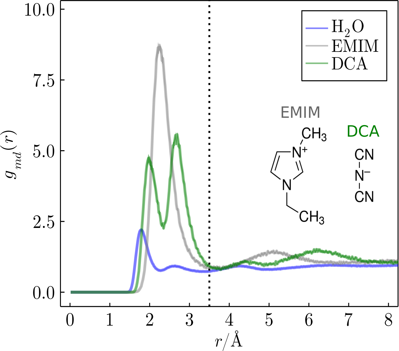
The algorithm is based on well-known methods for determining how long solvent molecules remain in each of a protein's solvation layers (references are given in Links 1 and 2). Using a molecular dynamics trajectory, the probability of a molecule remaining within the solvation shell of the protein is calculated, and the solvation shell can be defined by the minimum-distance distribution functions. In the above-displayed MDDFs, for instance, the most prominent peaks for the ions appear up to 4Å, indicating regions of the solution where the solvent molecules are more concentrated relative to the bulk.
The calculation is performed by defining a cutoff based on the distribution functions and determining whether a molecule is inside or outside the perimeter frame by frame - one if the molecule is inside, and zero if it is outside. The data is then stored in a matrix with dimensions equal to the number of frames (columns) and molecules (rows).
The figure below depicts the correlation function calculation process. Four snapshots from a simulation of molecular dynamics are illustrated. dt is a constant interval of time that separates every frame (time step of molecular dynamics). In the illustration, we are determining whether the water molecules are inside or outside the perimeter of dashed lines. The dashed line indicating the cut-off point will vary in shape for complex solutes because the distance we calculate is between one atom of the cosolvent (in this case, the O of water) and the nearest atom of the protein.
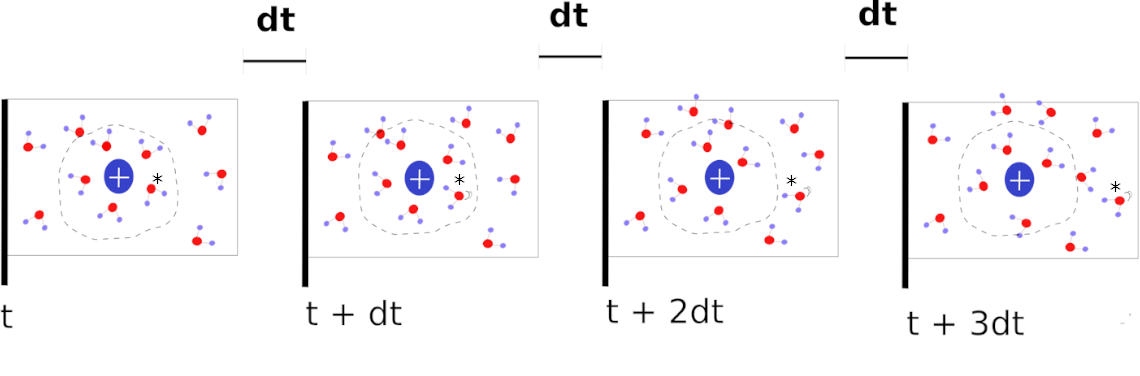
In the preceding example, the observed molecule (denoted by) is within the perimeter (dashed circle) at time t, and is therefore designated as 1. At time t + dt, the molecule is still within the boundary, but it is moving, so we mark it as 1. Consequently, we also number it. In frames 3 (t + 2dt) and 4 (t + 3dt), however, the molecule is outside the perimeter and is therefore represented by the value 0. The resulting matrix has the form [1 1 0 0], indicating that the molecule was within the perimeter analyzed in frames 1 and 2.
A molecule is considered to be in the evaluated region if it remains within the perimeter between times t and t + , where = ndt with n > 0. For 1 dt (1-time interval, we refer to it as dt1), the molecule was once contained within the perimeter. There was no time when the water stayed inside the perimeter for two, dt = 2 (dt 2), and three, dt = 3 (dt 3), time intervals following the first frame. Thus, given a value of dt, we generate a matrix containing the number of times the molecule stayed within the perimeter. The correlation matrix is transformed into [1 0 0]. This matrix indicates that the molecule remained inside the perimeter for the duration of dt 1 and did not reappear. Lastly, the sample space for the system is required to calculate the probability of survival. Thus, because we are dealing with four frames, we have the option of remaining within the evaluated region for three times the time dt1, twice the time dt2, and once the time dt3. Thus, [3 2 1] would be the sample space. As probability is the ratio of events to the sample space (correlation matrix), the result will be P = [1/3 0/2 0/1].
The data avaiable will be useful as an example for the way that ResTime.jl can be used to calculate time-correlation functions from molecular dynamics simulations
wget https://github.com/viniciuspiccoli/ResTime.jl/tree/master/data_example1/data.tar.gz
tar -xf archive.tar.gz
The files that will be used are the trajectory,sample-groMD.xtc, and the atoms' positions, sample-groMD.gro.
In this example, the time-correlation functions of EMIM, DCA, and water will be calculated until 3.5Å from the protein surface (vertical dotted line in the figure below). Minimum-distance distribution functions show that up to 3.5Å all relevant interactions with the protein already occurred, thus this distance will be used as a cutoff for the calculation.
Loading the packages required for the calculations:
using  Plots, LaTeXStrings
import Restime, PDBTools
To select the solute is necessary the usage of readPDB function from PDBTools, in this example, the solute is a protein. The first step is to load information about all atoms’ positions from a PDB (this PDB is the final frame of a simulation performed in gromacs).
solute  = "protein"
atoms   = PDBTools.readPDB("sample-groMD.pdb") # selection - all atoms of the PDB file.
After loading all atoms, it is necessary to select the protein atoms.
#protein selection
sel0    = PDBTools.select(atoms,solute)        # Selection of which atoms from the PDB are the protein atoms.
protein = ResTime.Selection(sel0, nmols=1)  # Selection for the calculation of time-correlation function / nmols = 1 (one protein)
Selection of solvent molecules. The calculation will use one atom for each solvent molecule. For instance, DCA is a molecule that contains 5 atoms (3 nitrogens and 2 carbons). For the time-corr calculation, it will be selected just the charged nitrogen. Therefore, performing the selection it is required the VMD nomenclature. Thus, to select the charged nitrogen of DCA the selection is name N3A and resname NC.
# anion selection
sel1    = PDBTools.select(atoms,"name N3A and resname NC")
anion   = ResTime.Selection(sel1,natomspermol=1)     # natomspermol = 1 - selection of 1 atom for each molecule

# cation selection
sel2    = PDBTools.select(atoms,"name LP and resname EMI")
cation  = ResTime.Selection(sel2,natomspermol=1)     # natomspermol = 1 - selection of 1 atom for each molecule
The oxygen selection from OPLS-AA TIP3P water can be done by:
# water selection
sel3    = PDBTools.select(atoms,"name OW and resname SOL")
water   = ResTime.Selection(sel3,natomspermol=1)     # natomspermol = 1 - selection of 1 atom for each molecule
Cutoff selection based on dotted line displayed at the MDDFs figure.
cutoff = 3.5 # cutoff based on MDDFs
Now, that all variables were definied, the trajecotry can be loaded doing:
trajectory = ResTime.Trajectory("trajectory.xtc", protein, anion, format="XTC" )
The correlation function, thus, can be computed using
time, prob = ResTime.correlation(trajectory, cutoff)
Print file to save data:
# Print the result in a file
ResTime.writefile("EMIMDCA","1.50",time_an, prob_an, prob_cat, prob_wat)
Example of the final result.
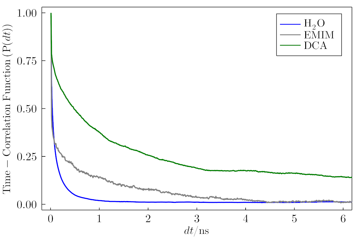
...