Data included in package
This package contains several example datasets that can be used to explore its functionality. The datasets and simulation scripts used to generate them are contained in their own dedicated branch, and described in detail below.
Once the data have been simulated, it is still incomplete - we must then estimate the individual treatment effects (ITEs) that are used to group observations. The description below also contains information on how the ITEs are estimated and subgroups determined.
-
Simple simulated data We describe in detail how to generate the simple simulated data included with the software.
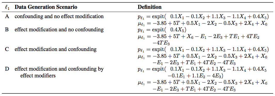
The table below defines the possible underlying correlation structures for the covariates in the simple simulated datasets.
-
Y~ N(mu, 1) is the continuous outcome, with the mean given in the table below. -
trt~ Bern(p) is the binary treatment, with the mean given in the table below. -
X5~ N(0,1) is a covariate associated with the treatment only (i.e., an instrument). -
X6~ N(0,1) is a covariate associate with the outcome only (i.e., a prognostic variable). -
X1,X2,X3,X4~i.i.d. N(0,1) are confounders of the effect of the treatment on the outcome. -
E1,E2, andE3~i.i.d. Bern(0.5) are binary effect modifiers that define eight subgroups within the data.
A dataset of size 1500 has been generated under each of the simulation scenarios, and is included upon installation of hetviz. Users are able to generate their own data under this general covariate structure using the function datagen() defined in simpleData.R. This function allows the user to generate a new sample under the population parameters given in the figure above, or specify their own as vectors:
## PSEUDOCODE

# coefficients for the treatment mean
#   should be given in the following order, in a
#   vector of length 9
alpha <- c(intercept, X1, X2, X3, X4, X5, E1, E2, E3)
# the data were generated using
alpha <- c(0, 0.1, -0.1, 1.1, -1.1, 0.4, -0.1, 1.1, -4)

# coefficients for the outcome mean
#   should be given in the following order, in a
#   vector of length 13
beta <- c(intercept, trt, X1, X2, X3, X4, X6, E1, E2, E3, TE1, TE2, TE3)
# the data were generated using
beta <- c(-3.85, 5, 0.5, -2, -0.5, 2, 1, -1, 0, -2, 1, 4, -4)Contained in simpleDataA.csv and generated by calling
datagen(n = 1500, effMod = FALSE, confound = TRUE, confoundEMs = FALSE)Contained in simpleDataB.csv and generated by calling
datagen(n = 1500, effMod = TRUE, confound = FALSE, confoundEMs = FALSE)Contained in simpleDataC.csv and generated by calling
datagen(n = 1500, effMod = TRUE, confound = TRUE, confoundEMs = FALSE)Contained in simpleDataD.csv and generated by calling
datagen(n = 1500, effMod = TRUE, confound = TRUE, confoundEMs = TRUE)BayesTree::bart() is used to estimate ITEs. After estimating the ITEs, their quantiles are used to partition the data into subgroups.
An example of how to do is is provided in simpleData.R.
After you have cleaned your data and constructed a variable indicating which subgroup each observation belongs to, you can provide this analytic dataset to hetviz under the "User-provided data" option.
- At minimum, a user-provided dataset requires a outcome variable (can be continuous or binary), a treatment variable (should be binary), and a variable that identifies hat subgroup each observation belongs to (preferably integer-valued). Details about the required data structure can be found in Data Provision.
The script complexData-medicareSim.R describes data simulated to mimic a real data set. These data are contained in complexData-medicareSim.csv, and can also be accessed using the "Complex simulated data" option of hetviz.