Basic analyses
Background
Absolute abundance VS relative abundance
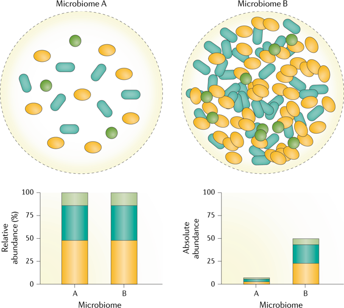
Due to DNA amplification and uneven sequencing depth, microbiome studies using amplicon sequences (i.e., 16s rRNA, ITS) are measuring relative abundance most times.
Data normalization, data transformation
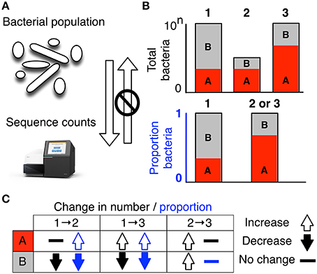
FIGURE 1. High-throughput sequencing data are compositional. (A) illustrates that the data observed after sequencing a set of nucleic acids from a bacterial population cannot inform on the absolute abundance of molecules. The number of counts in a high throughput sequencing (HTS) dataset reflect the proportion of counts per feature (OTU, gene, etc.) per sample, multiplied by the sequencing depth. Therefore, only the relative abundances are available. The bar plots in (B) show the difference between the count of molecules and the proportion of molecules for two features, A (red) and B (gray) in three samples. The top bar graphs show the total counts for three samples, and the height of the color illustrates the total count of the feature. When the three samples are sequenced we lose the absolute count information and only have relative abundances, proportions, or “normalized counts” as shown in the bottom bar graph. Note that features A and B in samples 2 and 3 appear with the same relative abundances, even though the counts in the environment are different. The table below in (C) shows real and perceived changes for each sample if we transition from one sample to another.
Compositionality of the data & CLR (Central log-ratio transformation)
Resources:
https://academic.oup.com/bioinformatics/article/34/16/2870/4956011 https://www.frontiersin.org/articles/10.3389/fmicb.2017.02224/full https://www.sciencedirect.com/science/article/pii/S1047279716300734?casa_token=YGK32CYqeTsAAAAA:IR19If3X29tjhwB5exvwuxOmROAso2VeFDl_DyQMl0Ju4prNDoYkUNt-OvteQu9pOppGVdOd
Alpha diversity
Alpha diversity (α-diversity) is defined as the mean diversity of species in different sites or habitats within a local scale.
Different alpha diversity measures
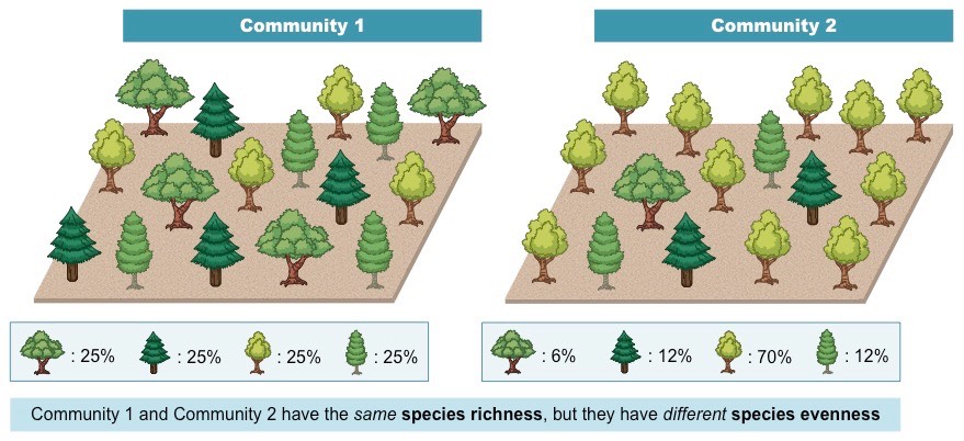
Richness and Evenness
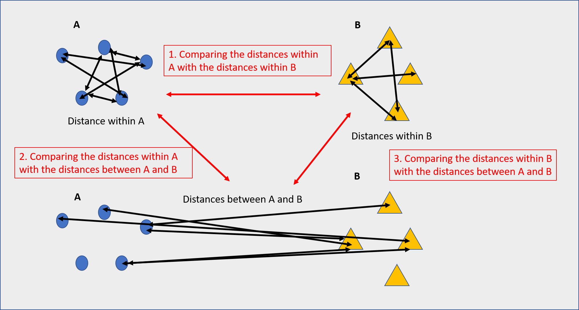
Beta diversity beta diversity is a measure of the similarity or dissimilarity of two communities distance between samples based on their similarity

Permutational multivariate analysis of variance (PERMANOVA) using beta diversity measures
Permutational multivariate analysis of variance (PERMANOVA) is a non-parametric multivariate statistical test. It compares groups of objects and tests the null hypothesis that the centroids and dispersion of the groups as defined by measure space are equivalent for all groups.
Data preparation
Load phyloseq object to the R studio
setwd("~/scratch")
phyloseq_16s <- readRDS("ps_16s.rds")
phyloseq_16s_filt <- subset_taxa(phyloseq16s, domain == "Bacteria") ### Filtering out non-bacterial ASVs
i) convert phyloseq object into designated level of taxonomy (genus)
library(phyloseq)
rank_names(phyloseq_16s_filt) # check the taxonomy structure
phyloseq_genus <- tax_glom(phyloseq_16s, taxrank = "genus") # combine ASVs into genus level
phyloseq_genus_rel <- transform_sample_counts(phyloseq_genus, function(x) x/sum(x)) # convert data into relative abundance
phyloseq_genus_rel_melt <- psmelt(phyloseq_genus_rel) # melt data
str(phyloseq_genus_rel_melt) # check the data structure
phyloseq_genus_rel_melt[,"genus"] <- as.character(phyloseq_genus_rel_melt[,"genus"])
phyloseq_genus_rel_melt[,"genus"][phyloseq_genus_rel_melt$Abundance < 0.1] <- "Other" #convert low abundance taxa (< 0.1) into "Other"
ii) Check how many genus in your dataset after converting low abundance taxa into "Others"
Count = length(unique(phyloseq_genus_rel_melt[,"genus"]))
if (Count > 25) {
  print("Warning: You have more than 25 taxa to plot, consider using higher cut off")
} else {
  print(Count)
}
iii) Sample Annotation with numbers (optional) First thing I would like to do is to add numbers to the bar with same color, to make if interpretable
phyloseq_genus_rel_melt$sample_order <- phyloseq_genus_rel_melt[,"genus"]
phyloseq_genus_rel_melt$sample_order <- as.factor(phyloseq_genus_rel_melt$sample_order)
levels(phyloseq_genus_rel_melt$sample_order) <- seq(1:length(levels(phyloseq_genus_rel_melt$sample_order)))
phyloseq_genus_rel_melt$text <- paste0(phyloseq_genus_rel_melt[,"genus"], "(", phyloseq_genus_rel_melt$sample_order,")")
#add numbers next to the genus name based on the alphabetic order
head(phyloseq_genus_rel_melt$text)

#getting color code for ploting - randomly assigned color
phyloseq_genus_rel_melt[,"genus"] <- as.factor(phyloseq_genus_rel_melt[,"genus"])
library(RColorBrewer)
qual_col_pals = brewer.pal.info[brewer.pal.info$category =='qual',]
col_vector <- unlist(mapply(brewer.pal, qual_col_pals$maxcolors, rownames(qual_col_pals)))
col=sample(col_vector, Count)

#Aggregate all relative abundacneb based on the group
phyloseq_genus_rel_melt_aggr <- aggregate(Abundance ~ Sample+text+sample_order+Type_of_sample+genus,
                                          data = phyloseq_genus_rel_melt, FUN=sum)
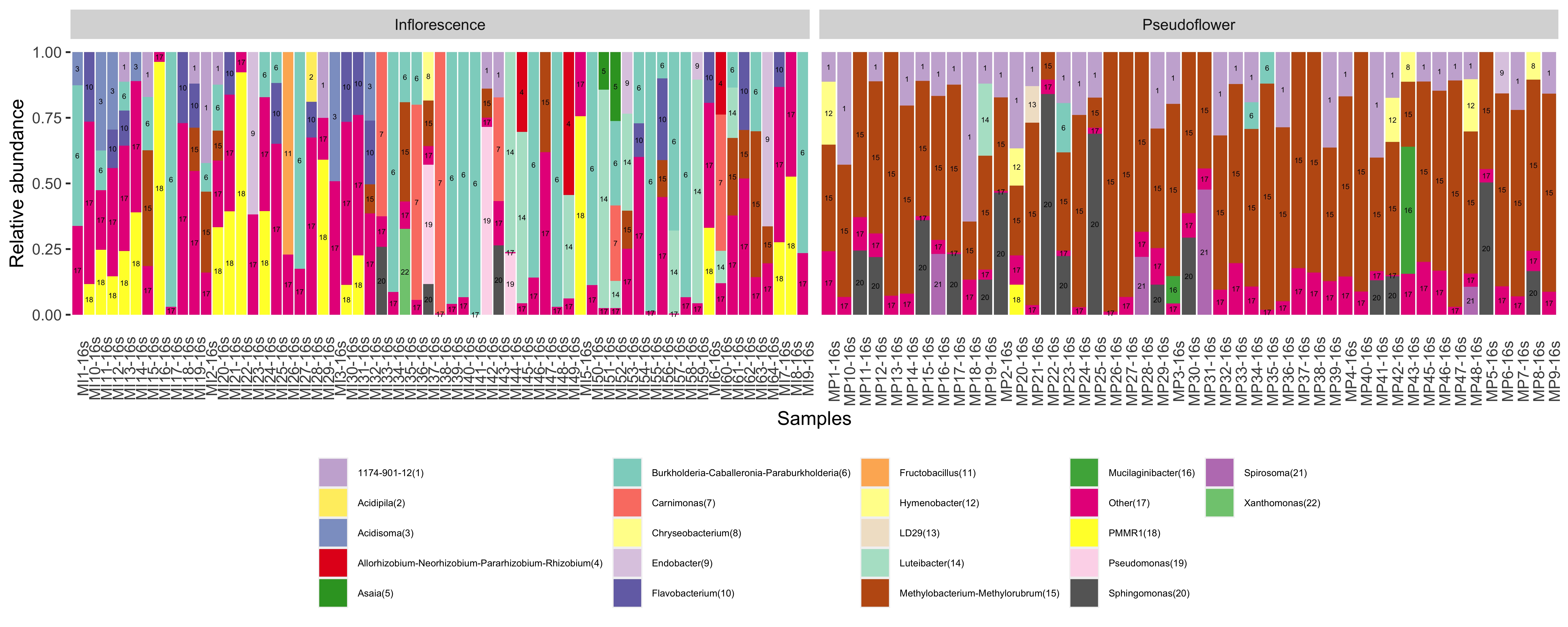
iv) plot stacked barplot
library(ggplot2)
plot <- ggplot(data=phyloseq_genus_rel_melt_aggr, aes(x=Sample, y=Abundance, fill= text)) +
  geom_bar(stat="identity", position="stack") +
  facet_grid(.~Type_of_sample, scales= "free") +
  guides(fill=guide_legend(nrow=5)) +
  scale_fill_manual(values=col)+
  theme(legend.position = "bottom", axis.text.x = element_text(angle=90),
        axis.ticks.x = element_blank(),
        panel.background = element_blank(),
        legend.title = element_blank()) +
  xlab("Samples") +
  ylab("Relative abundance") +
  geom_text(aes(label=sample_order), size = 1.5, position = position_stack(vjust = 0.5)) +
  theme(legend.text=element_text(size=5.5))
plot
ggsave("stacked_bar_plot_with_numbers.jpg", plot=plot, width = 12.5, height= 5, units = "in", dpi = 600)
Check the results --
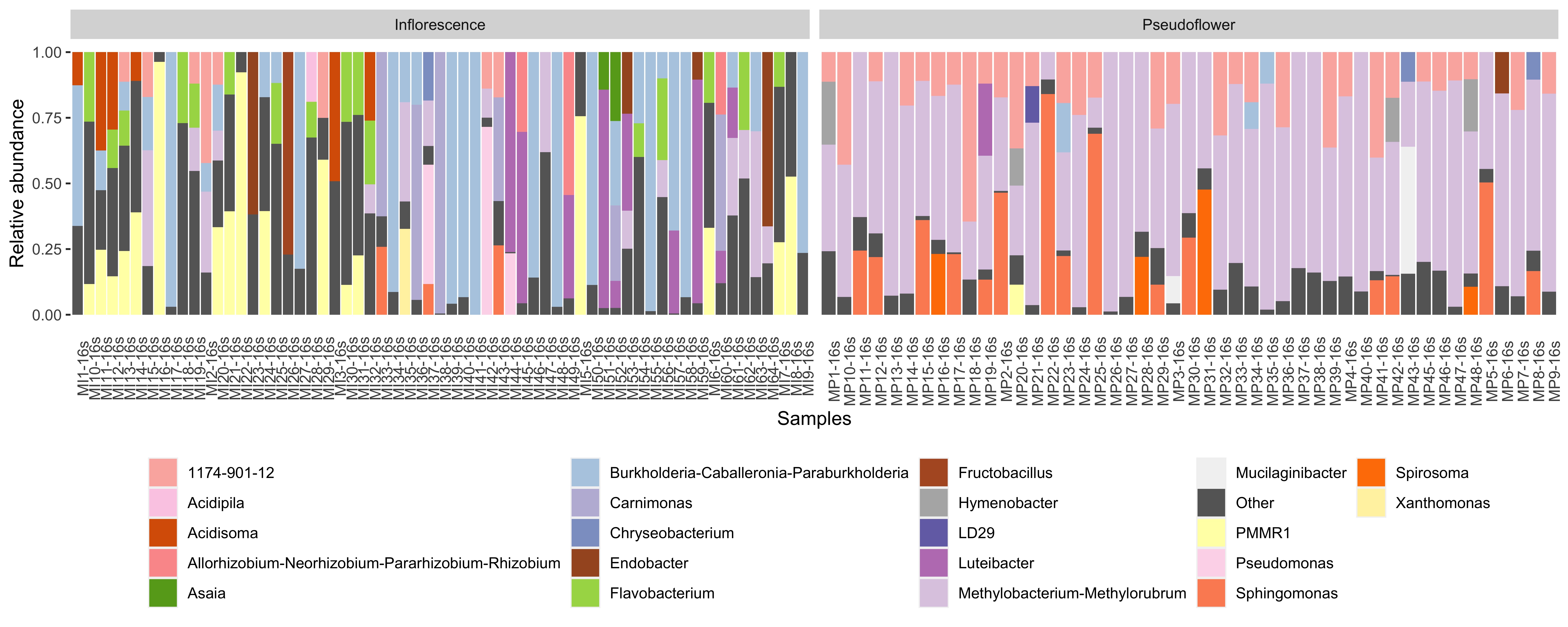
iv-2)plot without annotated numbers
plot_without_numbers <- ggplot(data=phyloseq_genus_rel_melt, aes(x=Sample, y=Abundance, fill= genus)) +
  geom_bar(stat="identity", position="stack") +
  facet_grid(.~Type_of_sample, scales= "free") +
  guides(fill=guide_legend(nrow=5)) +
  scale_fill_manual(values=col)+
  theme(legend.position = "bottom", axis.text.x = element_text(angle=90),
        axis.ticks.x = element_blank(),
        panel.background = element_blank(),
        legend.title = element_blank()) +
  xlab("Samples") +
  ylab("Relative abundance")
plot_without_numbers
ggsave("stacked_bar_plot_without_numbers.jpg", plot=plot_without_numbers, width = 12.5, height= 5, units = "in", dpi = 600)
library(ggpubr)
library(reshape2)
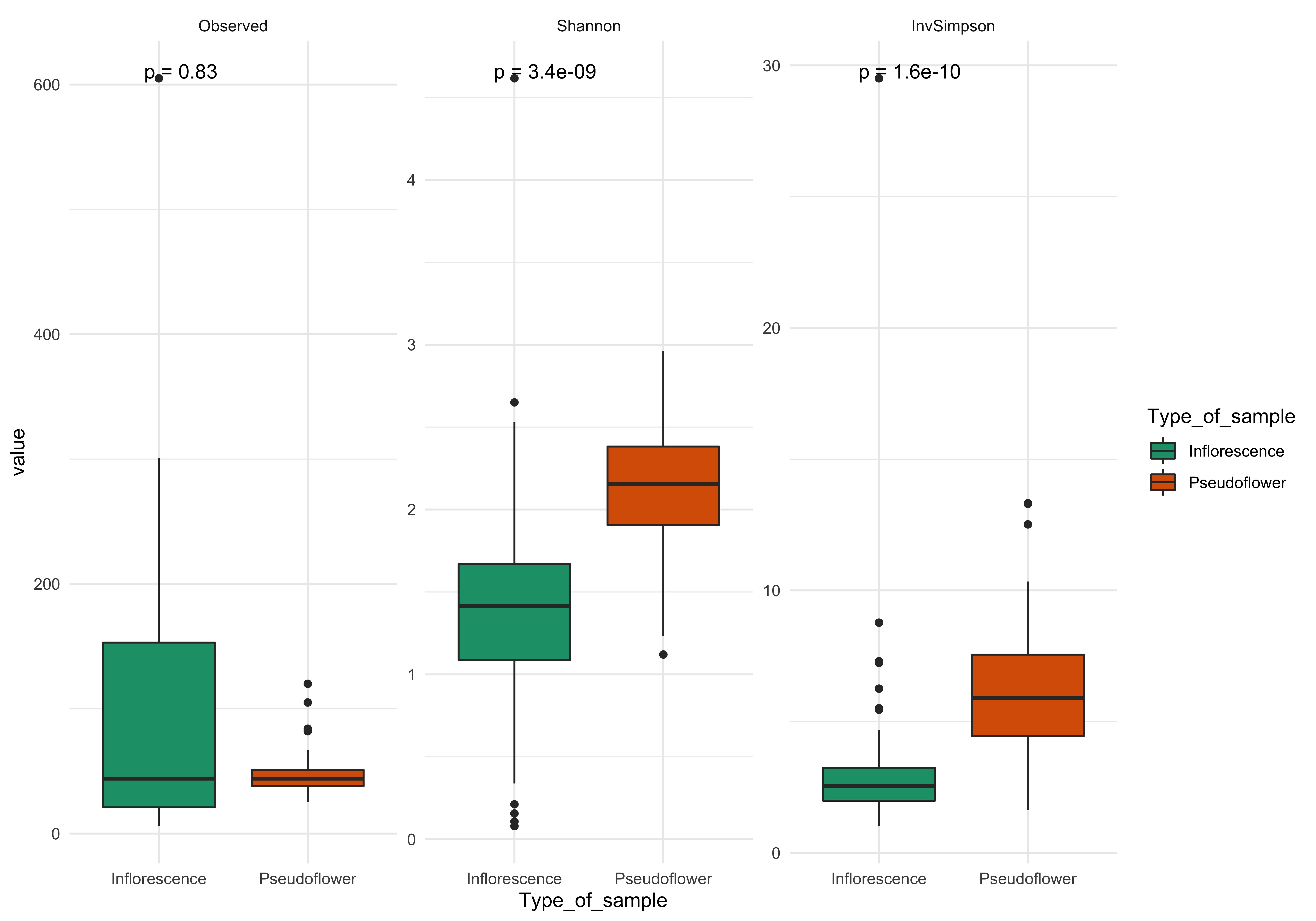
alpha_diversity <- estimate_richness(phyloseq_16s_filt, measures= c("Observed", "Shannon", "InvSimpson")) # calculate alpha diversity of selected measures
alpha_comparison <- cbind(alpha_diversity, sample_data(phyloseq_16s_filt)) # add metadata to the alpha diversity output
melt_plot <- melt(alpha_comparison) # melt data for plotting
plot_alpha <- ggplot(data = melt_plot, aes(y = value, x = Type_of_sample, fill = Type_of_sample)) +
geom_boxplot() +
facet_wrap(~variable, scale="free") +
theme_minimal() +
scale_fill_brewer(palette="Dark2") +
stat_compare_means(label = "p.format") # wilcox test (non-parametric test) for significance
plot_alpha
ggsave("alpha_diversity.jpg", plot = plot_alpha, width = 10, height=7, units= "in", dpi =600)
i) Data transformation (CLR - Central Log Ratio transformation)
#Following step requires samples on rows and ASVs in columns
otus <- otu_table(phyloseq_genus)
taxa_are_rows(otus) # Should be "FALSE" if "TRUE" use this command to transpose matrix "otus <- t(otus)"
#Replace zero values before clr transformation
#Use CZM method to replace zeros and outputs pseudo-counts (1)
require(zCompositions)
otu.n0 <- t(cmultRepl(otus, label =0, method="CZM", output="p-counts"))
otu.n0 <-ifelse(otu.n0 < 0, otu.n0*(-1), otu.n0)
#Convert data to proportions
otu.n0_prop <- apply(otu.n0, 2, function(x) {x/sum(x)})
#CLR transformation
otu.n0.clr<-t(apply(otu.n0_prop, 2, function(x){log(x)-mean(log(x))}))
phyloesq_genus_CLR <- phyloseq(otu_table(otu.n0.clr, taxa_are_rows=F),
                               tax_table(phyloseq_genus),
                               sample_data(phyloseq_genus))
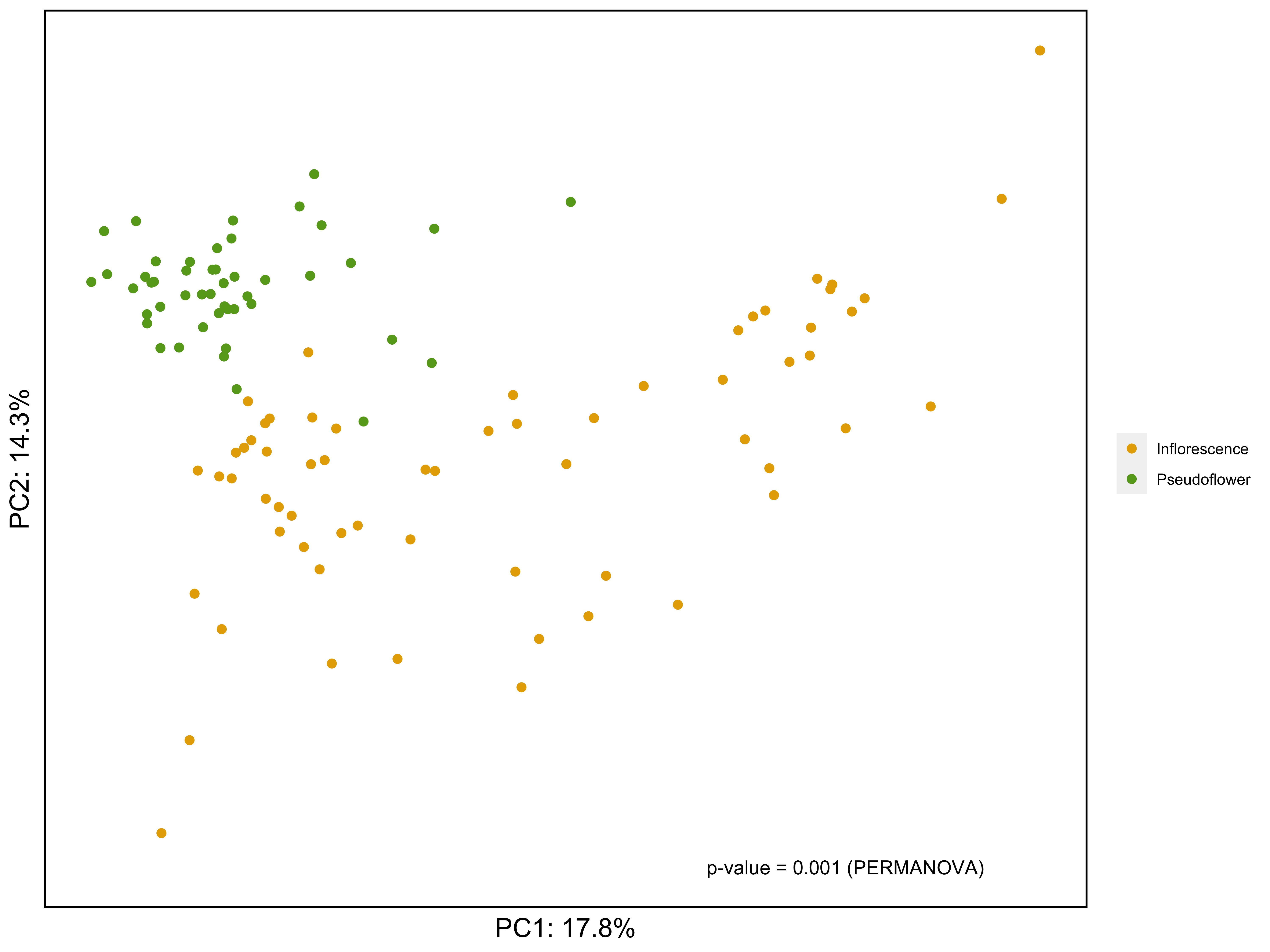
ii) PCA ordination with euclidean distance AND PERMANOVA (Permutation ANOVA)
#PCA
pc.clr <- prcomp(otu.n0.clr)
require(compositions)
# Calculate total variance (necessary for calculating %variance explained)
mvar.clr <- mvar(otu.n0.clr)
row <- rownames(otu.n0.clr)
# extract first two PCs
pc_out <- as.data.frame(pc.clr$x[,1:2])
# combine first two PCs with metadata
pc_out_meta <- as.data.frame(cbind(pc_out, sample_data(phyloesq_genus_CLR)))

# Calculate euclidean distance between sample
dist <- dist(otu.n0.clr, method = "euclidean")

# PERMANOVA (Permutational based ANOVA)
# https://onlinelibrary.wiley.com/doi/full/10.1002/9781118445112.stat07841
permanova <- vegan::adonis2(dist~Type_of_sample, data=pc_out_meta, perm =999)
permanova # Check PERMANOVA results
label = paste0("p-value = ",permanova$`Pr(>F)`[1]," (PERMANOVA)") #prepare label for plot
label # Check p-value

#Getting colors based on your comparisons
qual_col_pals = brewer.pal.info[brewer.pal.info$category =='qual',]
col_vector <- unlist(mapply(brewer.pal, 8, "Dark2"))
col=sample(col_vector, length(unique(pc_out_meta[,"Type_of_sample"])))

#Making PCA plot
PCA_plot <- ggplot(pc_out_meta, aes(x=PC1, y=PC2, color = Type_of_sample)) +
  geom_point(size=2)+
  theme(legend.position = 'right')+
  theme(axis.text = element_blank(), axis.ticks = element_blank()) +
  theme(axis.title = element_text(size=15,color='black')) +
  theme(panel.background = element_rect(fill='white', color = NA),
        plot.background = element_rect(fill = 'white',color = NA),
        panel.border = element_rect(color='black',fill = NA,size=1))+ # edit backgroud
  scale_x_continuous(name = paste("PC1: ", round(pc.clr$sdev[1]^2/mvar.clr*100, digits=1), "%", sep="")) + # %variance explained for PC1
  scale_y_continuous(name = paste("PC2: ", round(pc.clr$sdev[2]^2/mvar.clr*100, digits=1), "%", sep="")) + # %variance explained for PC2
  scale_color_manual(values= col) +
  theme(legend.title = element_blank()) +
  annotate("text", x = 15, y =-25, label = label) # Add PERMANOVA results to the plot
PCA_plot
ggsave("pca.jpg", plot = PCA_plot, width= 10, height=7.5, units="in", dpi=600)