Data processing (DADA2)

Background

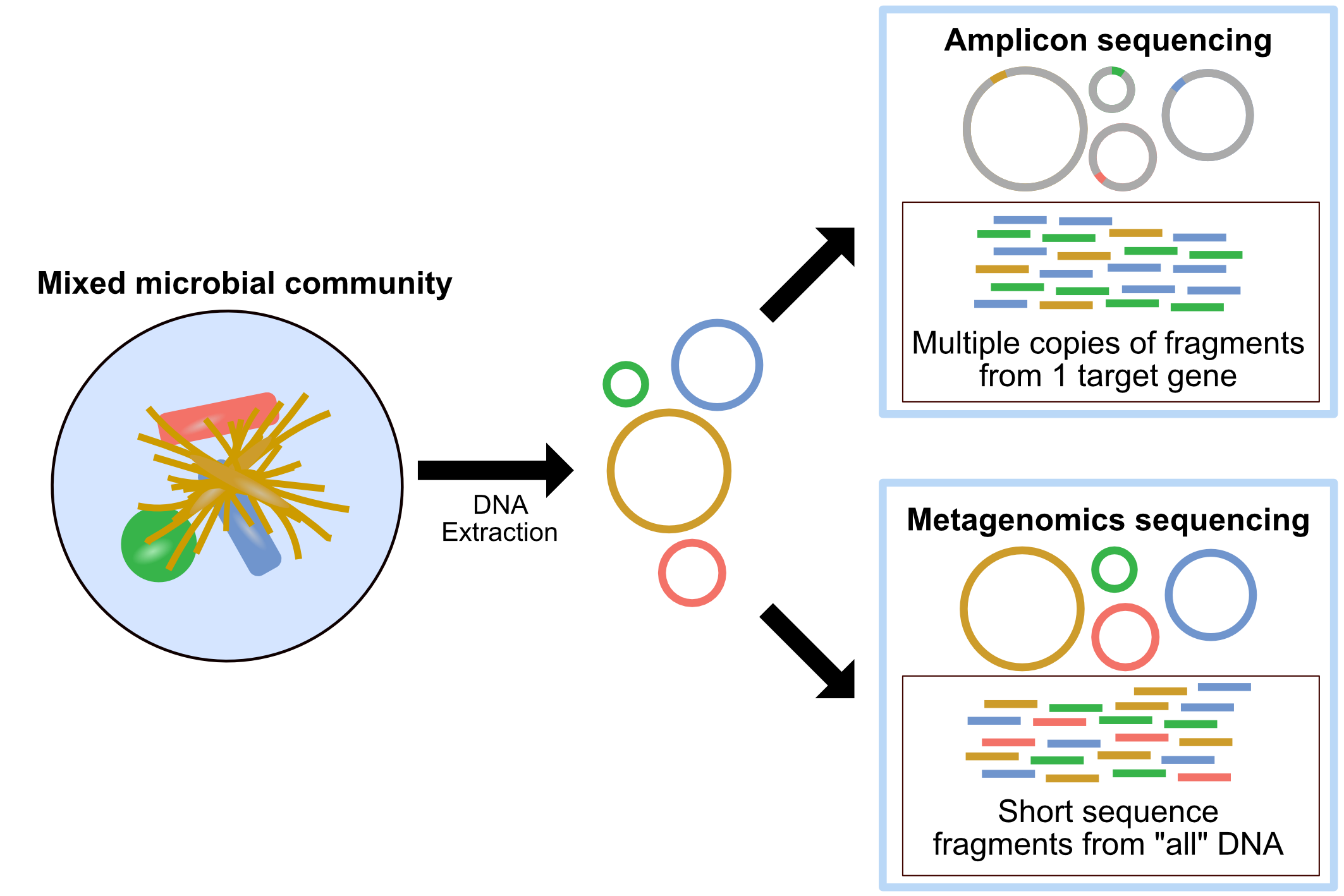
Type of sequencing

Amplicon sequencing Amplicon sequencing of marker-genes (e.g. 16S, 18S, ITS) involves using specific primers that target a specific gene or gene fragment. It is used for taxonomic classification and community structure changes in response to a treatment, environmental gradients and time. Also, this technology can focus on microbial DNAs extracted from sample (avoid host DNA contamination)

Metagenomics Shotgun metagenomic sequencing aims to amplify all the accessible DNA of a mixed community. It uses random primers and therefore suffers much less from pcr bias. Metagenomics provides a window into the taxonomy and functional potential of a sample. However, it takes more data to complete, and if your sample contains complicated host DNA, one would end up discarding too much data

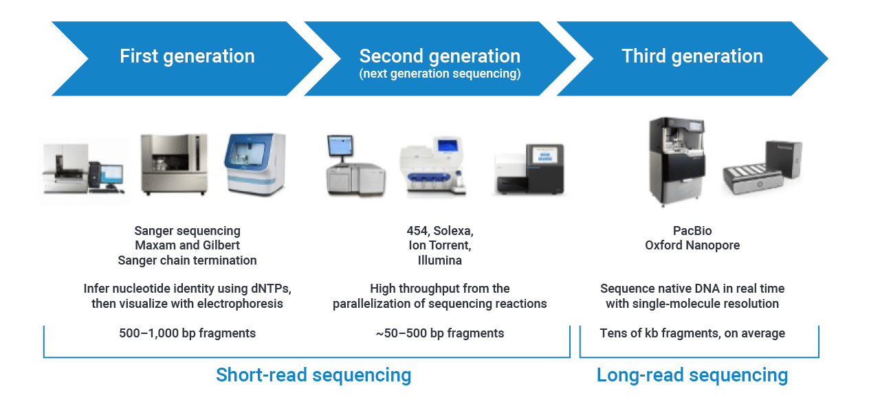
Sequencing platform

Sampling strategy and collection metadata

1. What is your comparison (continuous value? groups? treatment? spatial and/or temporal variations?)
2. How many samples will be collected?
3. Including controls (i.e., DNA extraction control, sampling control, library control, etc..)

General pipeline of microbiome study

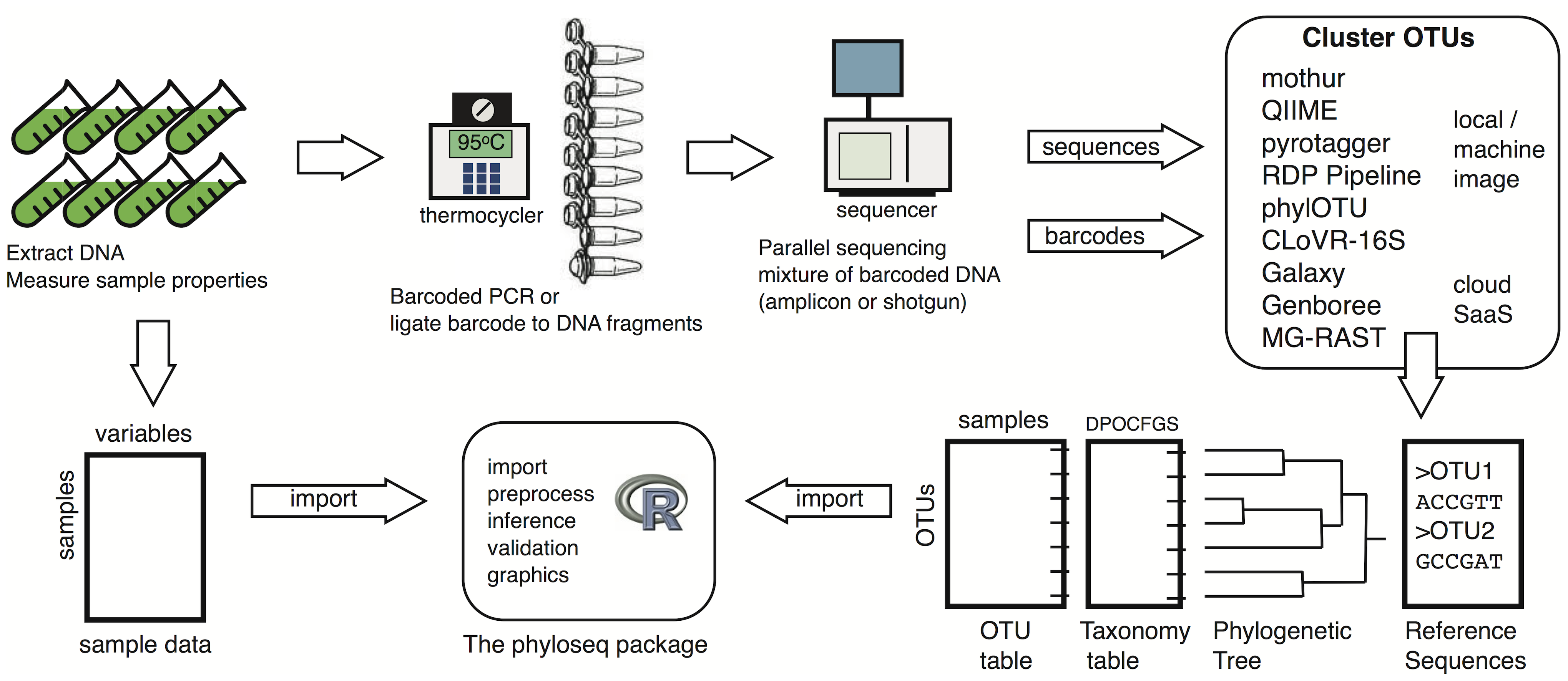
1. Sampling
2. DNA extraction/Library preparation
3. Sequencing
4. Data generation
5. Downstream analysis

More information about Microbiome center KickStart Workshop at https://github.com/Penn-State-Microbiome-Center/KickStart-Workshop-2022

DADA2 pipeline

What is DADA2?

Divisive Amplicon Denoising Algorithm (DADA) Fast and accurate sample inference from amplicon data with single-nucleotide resolution.

For detailed explanation - https://benjjneb.github.io/dada2/

Pipeline overview with annotation

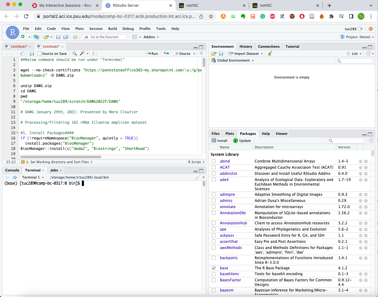
1. Install Packages If you already install those packages before coming to workshop, please skip this step

if (!requireNamespace("BiocManager", quietly = TRUE))
  install.packages("BiocManager")
BiocManager::install(c("dada2", "Biostrings", "ShortRead")
library(dada2)
library(Biostrings)
library(ShortRead)

2. Install optional bioinformatics program cutadapt (https://cutadapt.readthedocs.io/en/stable/) Cutadapt finds and removes adapter sequences, primers, poly-A tails and other types of unwanted sequence from your high-throughput sequencing reads.

1. Go to terminal (Linux command-line interpreter)

2. Download cutadapt using pip3 (the package installer for Python)

pip3 install --user --upgrade cutadapt

3. Check the path of installation of cutadapt

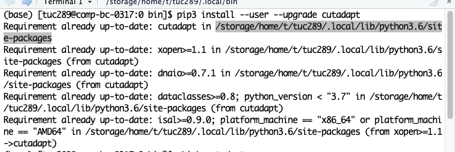
Copy that part to the script

3. Set working directory and identify file paths

1. Go to terminal (Linux command-line interpreter)

2. Download fastq files to your 'scratch' directory "All of the active storage is available from all of the Roar systems. Individual users have home, work and scratch directories that are created during account creation. The work and scratch directories should have links within the home directory, allowing for easy use. A user’s home directory is for personal files and cannot be shared. Work and scratch are able to be shared. Both home and work are backed up. Scratch is not backed up and files are subject to deletion 30 days after creation. Do not keep important files on scratch."

cd ~/scratch    # move to your own scratch directory
wget --no-check-certificate "https://pennstateoffice365-my.sharepoint.com/:u:/g/personal/tuc289_psu_edu/ESbdgUo93X1HgdMFsDNpo-sB0YiZ-UApG4RXrAtJOSYSDw?e=zRrTF5
&download=1" -O DAWG.zip    # download .zip file containing our sequences
unzip DAWG.zip    # decompress .zip file
cd DAWG     # move to the directory with files
ls     # check if you can see the list of files
pwd     # copy the output of this command - your file directory

4. Processing/filtering 16S rRNA Illumina amplicon dataset

1. Set Working directory

setwd("~/where your downloaded fastq files are")
path <- setwd("~/where your downloaded fastq files are")

2. Sort files

fnFs <- sort(list.files(path, pattern = "_R1_001.fastq.gz"))
fnRs <- sort(list.files(path, pattern = "_R2_001.fastq.gz"))

First you need to check your file name and their pattern

MI9-16s_S55_L001_R2_001.fastq.gz MP9-16s_S9_L001_R1_001.fastq.gz MP10-16s_S10_L001_R1_001.fastq.gz MP9-16s_S9_L001_R2_001.fastq.gz

Our files have R1_001. R2_002. pattern, but some other dataset might have different format (i.e, _1, _2 from NCBI SRA)

3. Getting sample names

sample.names <- sapply(strsplit(basename(fnFs), "_"), `[`,1)
sample.names

strsplit - string split, this command split character strings into multiple word based on the symbol "_"

4. Check for primers

FWD <- "GTGYCAGCMGCCGCGGTAA"
REV <- "GGACTACNVGGGTWTCTAAT"

You need to manually input your primer sequences (forward and reverse)

allOrients <- function(primer) {
  # Create all orientations of the input sequence
  require(Biostrings)
  dna <- DNAString(primer)  # The Biostrings works w/ DNAString objects rather than character vectors
  orients <- c(Forward = dna, Complement = complement(dna), Reverse = reverse(dna), 
        RevComp = reverseComplement(dna))
  return(sapply(orients, toString))  # Convert back to character vector
}
FWD.orients <- allOrients(FWD)
REV.orients <- allOrients(REV)
FWD.orients

Getting all different combination of primer sequences that can be found from your read

fnFs.filtN <- file.path(path, "filtN", basename(fnFs)) # Put N-filterd files in filtN/ subdirectory
fnRs.filtN <- file.path(path, "filtN", basename(fnRs))
filterAndTrim(fnFs, fnFs.filtN, fnRs, fnRs.filtN, maxN = 0, multithread = TRUE) # Filter all "N"s 

primerHits <- function(primer, fn) {
  # Counts number of reads in which the primer is found
  nhits <- vcountPattern(primer, sread(readFastq(fn)), fixed = FALSE)
  return(sum(nhits > 0))
}
rbind(FWD.ForwardReads = sapply(FWD.orients, primerHits, fn = fnFs[[1]]), 
   FWD.ReverseReads = sapply(FWD.orients, primerHits, fn = fnRs[[1]]), 
   REV.ForwardReads = sapply(REV.orients, primerHits, fn = fnFs[[1]]), 
   REV.ReverseReads = sapply(REV.orients, primerHits, fn = fnRs[[1]]))

Check how many primer sequences were hit to your files

Remove primers using cutadapt

cutadapt <- "/change to wherever cutadapt is located/cutadapt" 
system2(cutadapt, args = "--version")

path.cut <- file.path(path, "cutadapt")
if(!dir.exists(path.cut)) dir.create(path.cut)
fnFs.cut <- file.path(path.cut, basename(fnFs))
fnRs.cut <- file.path(path.cut, basename(fnRs))

FWD.RC <- dada2:::rc(FWD)
REV.RC <- dada2:::rc(REV)
# Trim FWD and the reverse-complement of REV off of R1 (forward reads)
R1.flags <- paste("-g", FWD, "-a", REV.RC) 
# Trim REV and the reverse-complement of FWD off of R2 (reverse reads)
R2.flags <- paste("-G", REV, "-A", FWD.RC) 
# Run Cutadapt
for(i in seq_along(fnFs)) {
  system2(cutadapt, args = c(R1.flags, R2.flags, "-n", 2, # -n 2 required to remove FWD and REV from reads
    "-o", fnFs.cut[i], "-p", fnRs.cut[i], # output files
    fnFs.filtN[i], fnRs.filtN[i])) # input files
}
# sanity check!
rbind(FWD.ForwardReads = sapply(FWD.orients, primerHits, fn = fnFs.cut[[1]]), 
   FWD.ReverseReads = sapply(FWD.orients, primerHits, fn = fnRs.cut[[1]]), 
   REV.ForwardReads = sapply(REV.orients, primerHits, fn = fnFs.cut[[1]]), 
   REV.ReverseReads = sapply(REV.orients, primerHits, fn = fnRs.cut[[1]]))

check detailed paramter for cutadapt from here - https://cutadapt.readthedocs.io/en/stable/guide.html

6. Check complexity and quality

plot(seqComplexity(getSequences(fnFs.cut[1])))
plot(seqComplexity(getSequences(fnRs.cut[1])))

plotQualityProfile(fnFs.cut[1:4])
plotQualityProfile(fnRs.cut[1:4])

• Currently plotting function in Rstudio server is not working properly in ROAR due to the Rstudio version issue. Here is the results from above commandlines

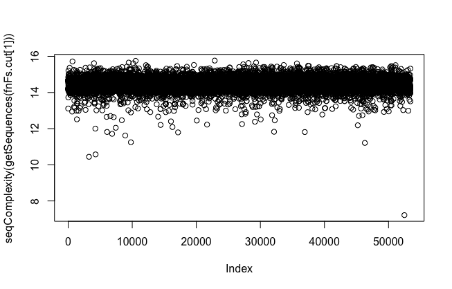
low-complexity reads are problematic. They will interfere when error rate calculates. Please consider using "rm.lowcomplex" function to remove low complex reads - but be careful, it might discard too many of your data

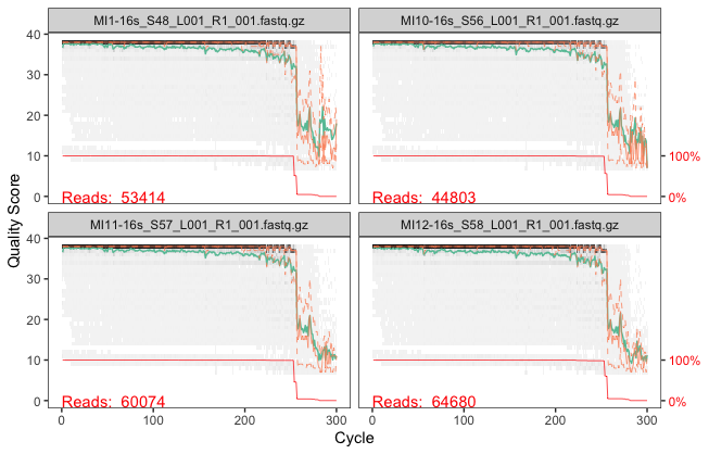
you can see from ~250bp, quality score drops notably. Let's consider this to filter and trim sequences in later part

7. Filter/Trim reads based on the quality metrics

filt_path <- file.path(path, "filtered")
if(!file_test("-d", filt_path)) dir.create(filt_path)
filtFs <- file.path(filt_path, paste0(sample.names, "_F_filt.fastq.gz"))
filtRs <- file.path(filt_path, paste0(sample.names, "_R_filt.fastq.gz"))

# Filter
for(i in seq_along(fnFs)) {
  fastqPairedFilter(c(fnFs.cut[i], fnRs.cut[i]), c(filtFs[i], filtRs[i]),
                    truncLen=c(240,160), 
                    maxN=0, maxEE=c(2,2), truncQ=2, rm.phix=TRUE,
                    compress=TRUE, verbose=TRUE)
}

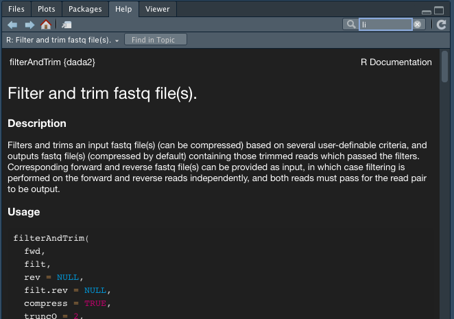
filterAndTrim paramters

?filterAndTrim

If you don't know what is phred scores (quality score) from fastq - https://support.illumina.com/help/BaseSpace_OLH_009008/Content/Source/Informatics/BS/QualityScoreEncoding_swBS.htm

8. Dereplication

derepFs <- derepFastq(filtFs, verbose=TRUE)
derepRs <- derepFastq(filtRs, verbose=TRUE)
# Name the derep-class objects by the sample names
names(derepFs) <- sample.names
names(derepRs) <- sample.names

Dereplication combines all identical sequencing reads into into “unique sequences” with a corresponding “abundance”: the number of reads with that same sequence. Dereplication substantially reduces computation time by eliminating redundant comparisons.

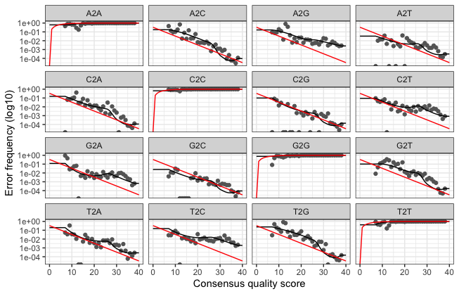
9. Learn the error rates

dadaFs.lrn <- dada(derepFs, err=NULL, selfConsist = TRUE, multithread=TRUE)
errF <- dadaFs.lrn[[1]]$err_out
dadaRs.lrn <- dada(derepRs, err=NULL, selfConsist = TRUE, multithread=TRUE)
errR <- dadaRs.lrn[[1]]$err_out

plotErrors(dadaFs.lrn[[1]], nominalQ=TRUE)

10. Sample Inference We are now ready to apply the core sequence-variant inference algorithm to the dereplicated data.

dadaFs <- dada(derepFs, err=errF, multithread=TRUE)
dadaRs <- dada(derepRs, err=errR, multithread=TRUE)
dadaFs[[1]]

11. Merge paired reads Merging forward and reverse reads

mergers <- mergePairs(dadaFs, derepFs, dadaRs, derepRs, verbose=TRUE)
# Inspect the merger data.frame from the first sample
head(mergers[[1]])

12. Constructing the sequence table - sequence counting table We can now construct a sequence table of our mouse samples that is analagous to the “OTU table” produced by classical methods.

seqtab <- makeSequenceTable(mergers[names(mergers) != "Mock"])
dim(seqtab)
table(nchar(getSequences(seqtab))) # Inspect distribution of sequence lengths

13. Remove chimeras

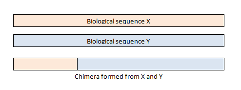
Chimeras are sequences formed from two or more biological sequences joined together. Amplicons with chimeric sequences can form during PCR. Chimeras are rare with shotgun sequencing, but are common in amplicon sequencing when closely related sequences are amplified. Although chimeras can be formed by a number of mechanisms, the majority of chimeras are believed to arise from incomplete extension. During subsequent cycles of PCR, a partially extended strand can bind to a template derived from a different but similar sequence. This then acts as a primer that is extended to form a chimeric sequence ([Smith et al. 2010], [Thompson et al., 2002], [Meyerhans et al., 1990], [Judo et al., 1998], [Odelberg, 1995]).

seqtab.nochim <- removeBimeraDenovo(seqtab, verbose=TRUE)
dim(seqtab.nochim)
sum(seqtab.nochim)/sum(seqtab)  # Check proportion of chmeric reads in the dataset

14. Assign taxonomy first we need to download database

# Run below in your terminal
wget https://zenodo.org/record/4587955/files/silva_nr99_v138.1_train_set.fa.gz?download=1 -O silva_nr99_v138.1_train_set.fa.gz
wget https://zenodo.org/record/4587955/files/silva_species_assignment_v138.1.fa.gz?download=1 -O silva_species_assignment_v138.1.fa.gz

set.seed(128)
taxa <- assignTaxonomy(seqtab.nochim, "silva_nr99_v138.1_train_set.fa.gz", multithread = TRUE)
taxa.species <- addSpecies(taxa, "silva_species_assignment_v138.1.fa.gz", verbose=TRUE)

15. Combine everything as one phyloseq object and save it in your computer

Install phyloseq package

BiocManager::install("phyloseq")
library(phyloseq)

Making phyloseq object https://joey711.github.io/phyloseq/

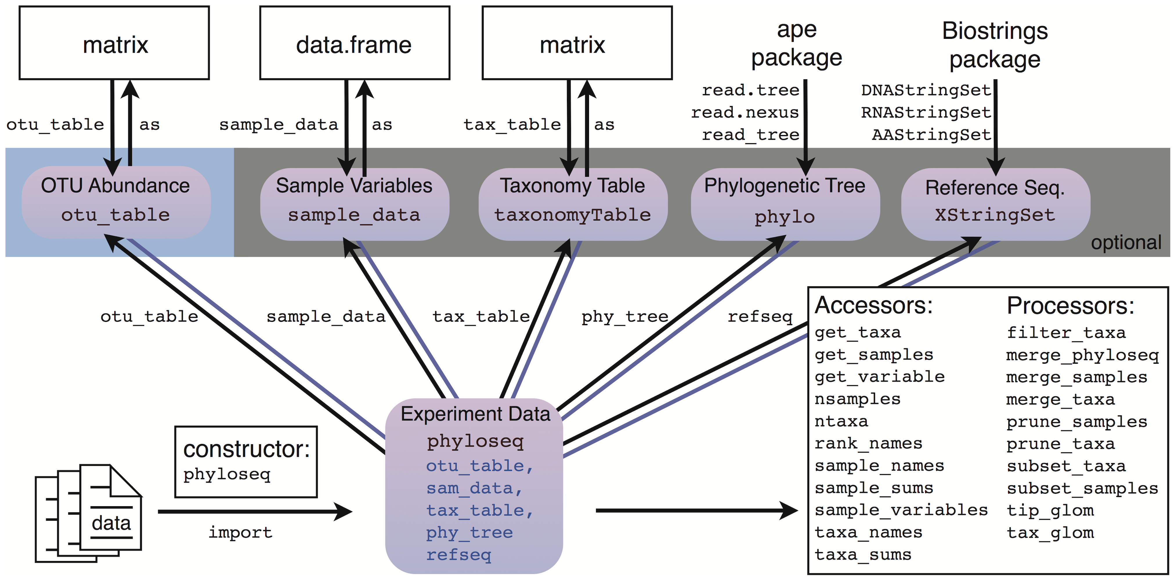
ps <- phyloseq(otu_table(seqtab.nochim), taxa_are_rows=FALSE),
               tax_table(taxa.species))
ps

Saving as .rds file

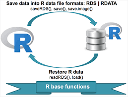
# Save an object to a file
saveRDS(ps, file = "phyloseq.rds")
# Restore the object
readRDS(file = "phyloseq.rds")

Saving entire environment as .rdata file

# Save entire environment to a file
save.image("dada2.Rdata")
load(file = "dada2.Rdata")